Setting up Swingbench for Oracle Autonomous Transaction Processing (ATP)
Step 1/ Make Sure you have a SSH Public key
You are likely to already have a ssh key but it is possible that you want to create another purely for this exercise. You’ll need this key to create your application server. You can find details on how to do this here
https://git-scm.com/book/en/v2/Git-on-the-Server-Generating-Your-SSH-Public-Key
It’s the .pub file or more precisely its contents that you’ll need. The public key file is typically created in the hidden .ssh directory in your home directory. The public key will look something like this (modified)
ssh-rsa AAAAB3NzaC1yc2EAAAADAQABAAABAQDfO/80wleUCYxY7Ws8c67PmqL2qRUfpdPGOduHmy9xT9HkCzjoZHHIk1Zx1VpFtQQM+RwJzArZQHXrMnvefleH20AvtbT9bo2cIIZ8446DX0hHPGaGYaJNn6mCeLi/wXW0+mJmKc2xIdasnH8Q686zmv72IZ9UzD12o+nns2FgCwfleQfyVIacjfi+dy4DB8znpb4KU5rKJi5Zl004pd1uSrRtlDKR9OGILvakyf87CnAP/T8ITSMy0HWpqc8dPHJq74S5jeQn/TxrZ6TGVA+xGLzLHN4fLCOGY20gH7w3rqNTqFuUIWuIf4OFdyZoFBQyh1GWMOaKjplUonBmeZlV
You’ll need this in step 3.
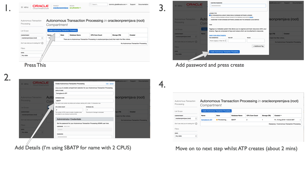
Step 2/ Create the ATP Instance
You’ll have to have gone through the process of acquiring an Oracle Cloud account but that’s beyond the scope of this walkthrough. Once you have the account and have logged into Oracle Cloud Infrastructure, click on the menu button in the top left of the screen and select “Autonomous Transaction Processing”. Then simply follow these steps.
Step 3/ Create a compute resource for the application server
Whilst the ATP instance is creating we can create our application to run swingbench. For any reasonable load to be run against the application server you’ll need a minimum of two cores for larger workloads you may need a bigger application or potentially a small cluster of them.
In this walkthrough we’ll create a small 2 core Linux Server VM.
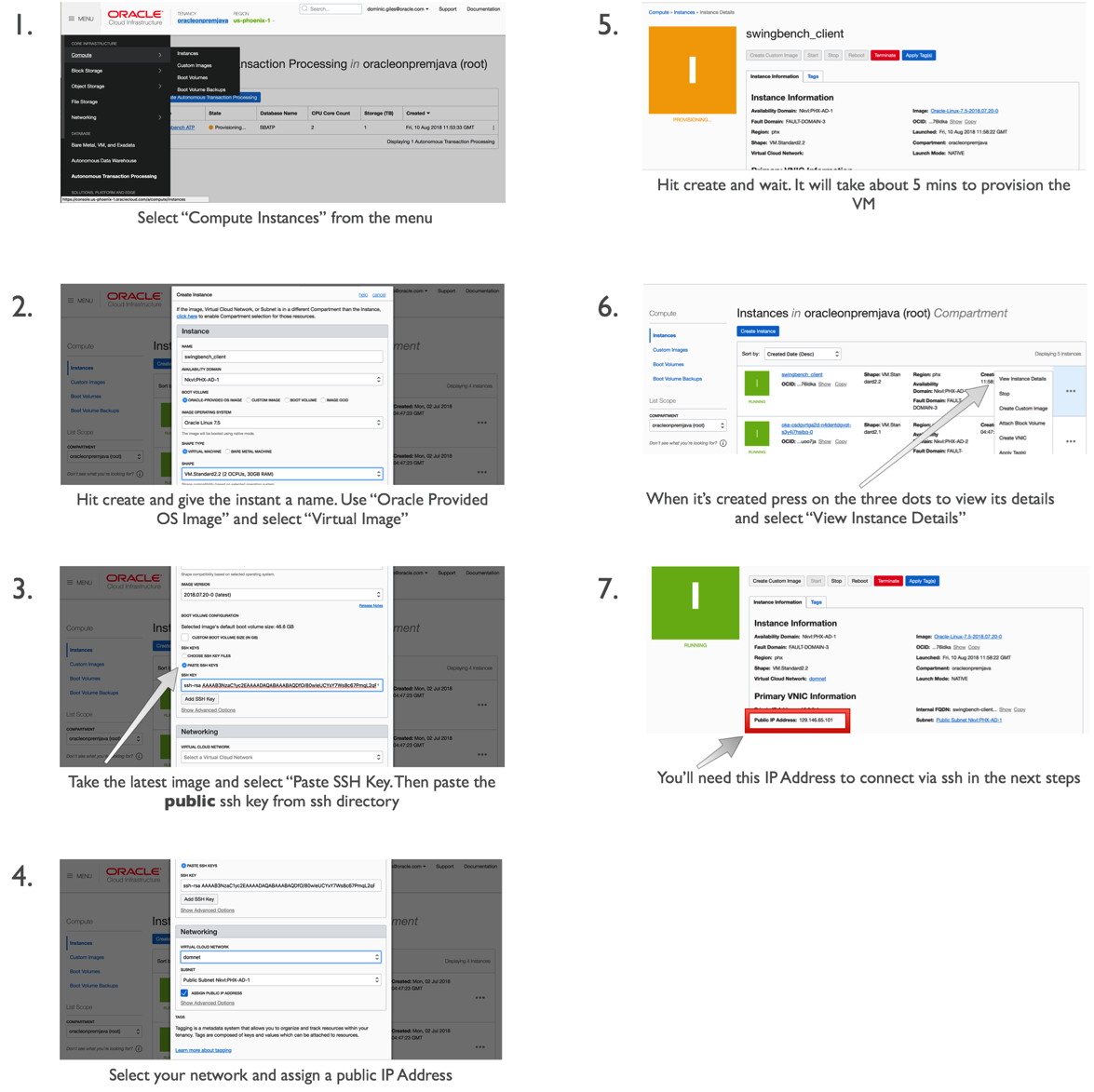
This should only take a couple of minutes. On completion we’ll need to use the public IP address of the application server we created in the previous step.
Step 4/ Log onto application server and setup the environment
In this step we’ll use ssh to log onto the application server and setup the environment to run swingbench. Ssh is natively available on MacOS and Linux. On platforms like Windows you can use Putty. You’ll need the IP address of the application server you created in the previous step.
First bring up a terminal on Linux/Mac. On Putty launch a new ssh session. The username will be “opc”
ssh opc@< IP Address of Appserver >
You should see something similar to
$> ssh opc@129.146.65.101
ECDSA key fingerprint is SHA256:kNbpKWL3M1wB6PUFy2GOl+JmaTIxLQiggMzn6vl2qK1tM.
Are you sure you want to continue connecting (yes/no)? yes
Warning: Permanently added '129.146.65.101' (ECDSA) to the list of known hosts.
Enter passphrase for key '/Users/dgiles/.ssh/id_rsa':
[opc@swingbench-client ~]$
By default java isn’t installed on this VM so we’ll need to install it via yum. We’ll need to update yum first
$> sudo yum makecache fast
Then we can install java and its dependencies
$> sudo yum install java-1.8.0-openjdk-headless.x86_64
We should now make sure that java works correctly
$> java -version
openjdk version "1.8.0_181"
OpenJDK Runtime Environment (build 1.8.0_181-b13)
OpenJDK 64-Bit Server VM (build 25.181-b13, mixed mode)
We can now pull the swingbench code from the website
$> curl http://www.dominicgiles.com/swingbench/swingbench261082.zip -o swingbench.zip
and unzip it
$> unzip swingbench.zip
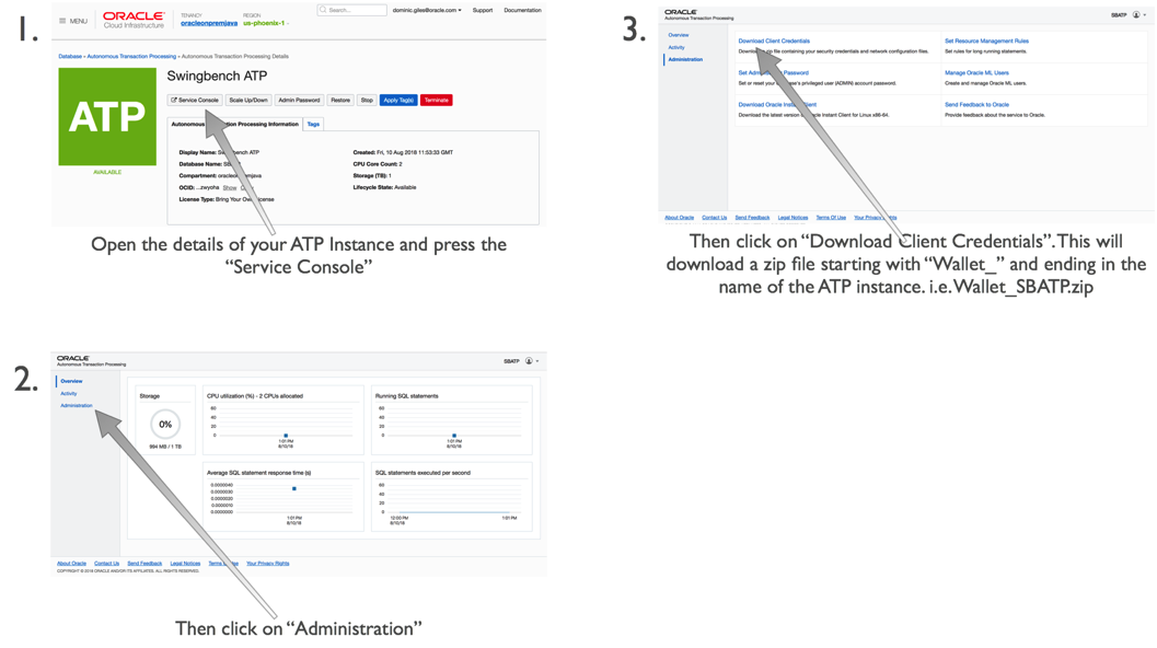
Step 5/ Download the credentials file
The next step is to get the credentials file for ATP. You can do this by following these steps.
You’ll need to upload this to our application server with a command similar to
$> scp wallet_SBATP.zip opc@129.146.65.101:
This will place our credentials file in the home directory of the application server. You don’t need to unzip it to use it.
Step 6/ Install a workload schema into the ATP instance
We can now install a schema to run our transactions against. We do this by first changing in to the swingbench bin directory
$> cd swingbench/bin
And then running the following command replacing your passwords with those that you specified during the creation of the ATP instance.
A quick explanation of the parameters we are using
- -cf tells oewizard the location of the credentials file
- -cs is the connecting for the service of the ATP instance. It is based on the name of the instance and is of the form
followed by one of the following _low, _medium,_high,_parallel - -ts is the name of the table space to install swingbench into. It is currently always “data”
- -dba is the admin user, currently this is always admin
- -dbap is the password you specified at the creation of the ATP instance
- -u is the name you want to give to the user you are installing swingbench into (I’d recommend soe)
- -p is the password for the user. It needs to follow the password complexity rules of ATP
- -async_off you need to disable the wizards default behavior of using async commits. This is currently prohibited on ATP
- -scale indicates the size of the schema you want to create where a scale of 1 will generate 1GB of data. The indexes will take an additional amount of space roughly half the size of the data. A scale of 10 will generate a 10GB of data and roughly of 5GB of indexes
- -hashpart tells the wizard to use hash partitioning
- -create tells swingbench to create the schema (-drop will delete the schema)
- -cl tells swingbech to run in character mode
- -v tells swingbench to output whats going on (verbose mode)
You should see the following output. A scale of 1 should take just over 5 mins to create. If you specified more CPUs for the application server of ATP instance you should see some improvements in performance, but this is unlikely to truly linear because of the nature of the code.
SwingBench Wizard
Author  :	 Dominic Giles
Version :	 2.6.0.1082

Running in Lights Out Mode using config file : ../wizardconfigs/oewizard.xml
Connecting to : jdbc : oracle : thin : @sbatp_medium
Connected
Starting run
Starting script ../sql/soedgdrop2.sql
Script completed in 0 hour(s) 0 minute(s) 2 second(s) 691 millisecond(s)
Starting script ../sql/soedgcreatetableshash2.sql
Script completed in 0 hour(s) 0 minute(s) 1 second(s) 433 millisecond(s)
Starting script ../sql/soedgviews.sql
Script completed in 0 hour(s) 0 minute(s) 0 second(s) 31 millisecond(s)
Starting script ../sql/soedgsqlset.sql
Script completed in 0 hour(s) 0 minute(s) 0 second(s) 196 millisecond(s)
Inserting data into table ADDRESSES_1124999
Inserting data into table ADDRESSES_2
Inserting data into table ADDRESSES_375001
Inserting data into table ADDRESSES_750000
Inserting data into table CUSTOMERS_749999
Inserting data into table CUSTOMERS_250001
Inserting data into table CUSTOMERS_500000
Inserting data into table CUSTOMERS_2
Run time 0:00:19 : Running threads (8/8) : Percentage completed : 5.36
You can then validate the schema created correctly using the following command
$> ./sbutil -soe -cf ~/wallet_SBATP.zip -cs sbatp_medium -u soe -p < a password for the soe user > -val
The Order Entry Schema appears to be valid.
--------------------------------------------------
|Object Type    |     Valid|   Invalid|   Missing|
--------------------------------------------------
|Table          |        10|         0|         0|
|Index          |        26|         0|         0|
|Sequence       |         5|         0|         0|
|View           |         2|         0|         0|
|Code           |         1|         0|         0|
--------------------------------------------------
You may have noticed that the stats failed to collect in the creation of the schema (known problem) so you’ll need to collect stats using the following command
$>./sbutil -soe -cf ~/wallet_SBATP.zip -cs sbatp_medium -u soe -p
And see the row counts for the tables with
$ ./sbutil -soe -cf ~/wallet_SBATP.zip -cs sbatp_medium -u soe -p < your soe password > -tables
Order Entry Schemas Tables
----------------------------------------------------------------------------------------------------------------------
|Table Name                  |                Rows|              Blocks|           Size|   Compressed?|  Partitioned?|
----------------------------------------------------------------------------------------------------------------------
|ORDER_ITEMS                 |           4,271,594|              64,448|        512.0MB|              |           Yes|
|ADDRESSES                   |           1,500,000|              32,192|        256.0MB|              |           Yes|
|LOGON                       |           2,382,984|              32,192|        256.0MB|              |           Yes|
|CARD_DETAILS                |           1,500,000|              32,192|        256.0MB|              |           Yes|
|ORDERS                      |           1,429,790|              32,192|        256.0MB|              |           Yes|
|CUSTOMERS                   |           1,000,000|              32,192|        256.0MB|              |           Yes|
|INVENTORIES                 |             897,672|               2,386|         19.0MB|      Disabled|            No|
|PRODUCT_DESCRIPTIONS        |               1,000|                  35|          320KB|      Disabled|            No|
|PRODUCT_INFORMATION         |               1,000|                  28|          256KB|      Disabled|            No|
|ORDERENTRY_METADATA         |                   4|                   5|           64KB|      Disabled|            No|
|WAREHOUSES                  |               1,000|                   5|           64KB|      Disabled|            No|
----------------------------------------------------------------------------------------------------------------------
                                                            Total Space           1.8GB
Step 7/ Run a workload
The first thing we need to do is to configure the load generator to load the users on in a sensible fashion (i.e. to not exceed the login rate). You could do this manually by editing the config file or use the following command.
We can now run a workload against the newly created schema using a command similar to
I won’t explain the parameters that I detailed earlier when running the wizard but for the new ones do the following
• -v indicates what info should be shown in the terminal when running the command. In this instance I’ve asked that the users logged on, Tx/Min, Tx/Sec and the average response time for each transaction are shown.
• -min and -max indicate the time to sleep between each DML operation in a transaction (intra sleep). A Transaction is made up of many DML operations
• -intermin -intermax indicates the time to sleep between each transaction.
• -di indicates that I want to disable the following transactions SQ,WQ,WA. These are reporting queries and aren’t really needed.
• -rt indicates how long to run the benchmark before stopping it
You should see output similar to the following
$> ./charbench -c ../configs/SOE_Server_Side_V2.xml -cf ~/wallet_SBATP.zip -cs sbatp_low -u soe -p < your soe password > -v users,tpm,tps,vresp -intermin 0 -intermax 0 -min 0 -max 0 -uc 128 -di SQ,WQ,WA -rt 0:0.30
Author  :	 Dominic Giles
Version :	 2.6.0.1082

Results will be written to results.xml.
Hit Return to Terminate Run...

Time		Users	TPM	TPS	NCR	UCD	BP	OP	PO	BO	SQ	WQ	WA
17:29:53	[0/128]	0	0	0	0	0	0	0	0	0	0	0
17:29:54	[0/128]	0	0	0	0	0	0	0	0	0	0	0
17:29:55	[0/128]	0	0	0	0	0	0	0	0	0	0	0
17:29:56	[40/128]	0	0	0	0	0	0	0	0	0	0	0
17:29:57	[45/128]	0	0	0	0	0	0	0	0	0	0	0
17:29:58	[51/128]	0	0	0	0	0	0	0	0	0	0	0
17:29:59	[60/128]	0	0	0	0	0	0	0	0	0	0	0
17:30:00	[69/128]	0	0	0	0	0	0	0	0	0	0	0
17:30:01	[78/128]	0	0	0	0	0	0	0	0	0	0	0
17:30:02	[84/128]	0	0	0	0	0	0	0	0	0	0	0
17:30:03	[95/128]	0	0	0	0	0	0	0	0	0	0	0
17:30:04	[101/128]	0	0	0	0	0	0	0	0	0	0	0
17:30:05	[104/128]	0	0	419	395	547	554	0	570	0	0	0
17:30:06	[108/128]	118	118	653	110	379	1576	375	647	0	0	0
17:30:07	[116/128]	325	207	355	220	409	406	499	450	0	0	0
17:30:08	[128/128]	547	222	423	100	203	504	403	203	0	0	0
17:30:09	[128/128]	831	284	420	306	303	396	501	505	0	0	0
17:30:10	[128/128]	1133	302	344	234	232	884	603	217	0	0	0
17:30:11	[128/128]	1438	305	564	367	355	375	559	376	0	0	0
17:30:12	[128/128]	1743	305	443	150	323	319	233	143	0	0	0
17:30:13	[128/128]	2072	329	1712	179	108	183	325	179	0	0	0
17:30:14	[128/128]	2444	372	1036	102	147	204	194	134	0	0	0
17:30:15	[128/128]	2807	363	1584	85	182	234	179	169	0	0	0
17:30:16	[128/128]	3241	434	741	159	157	250	256	251	0	0	0
17:30:17	[128/128]	3653	412	517	91	178	181	176	137	0	0	0
We specified a runtime of 30 seconds (-rt 0:0.30) which meant the workload ran for a short period of time. You could increase this by changing the the -rt parameter to something larger like
-rt 1:30
Which would run the benchmark for 1 hour 30mins. or you could leave the -rt command off altogether and the benchmark would run until you hit return.
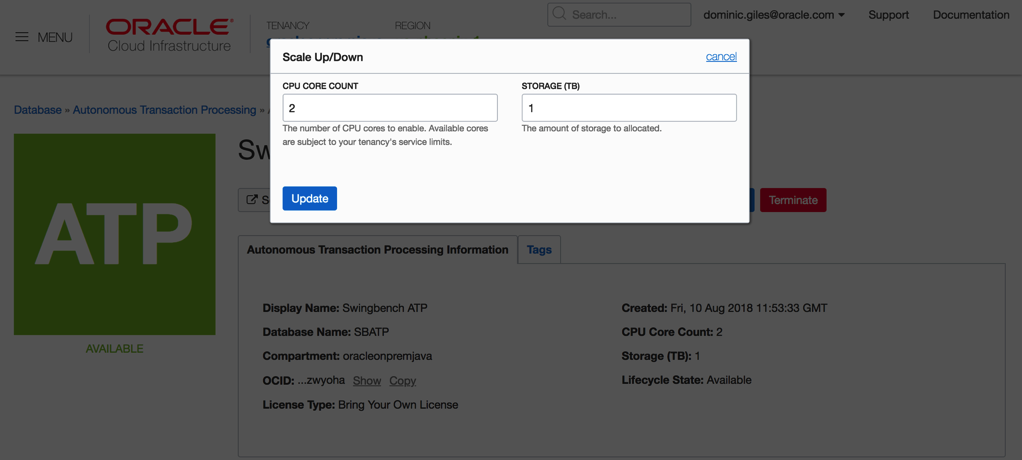
One thing to try whilst running the load against the server is to try and scale the number of available CPUs to the ATP instance up and down. This should see an increase in the number of transactions being processed.
Somethings to note. At the end of each run you’ll end up with a results file in xml format in the directory you ran charbench from. i.e.
$ ls
bmcompare  clusteroverview  debug.log   oewizard          results00003.xml  results00006.xml  results00009.xml  sbutil      swingbench
ccwizard   coordinator      jsonwizard  results00001.xml  results00004.xml  results00007.xml  results2pdf       shwizard    tpcdswizard
charbench  data             minibench   results00002.xml  results00005.xml  results00008.xml  results.xml       sqlbuilder
These xml files contain the detailed results of each run i.e. average transactions per second, completed transactions, percentile response times etc. Whilst these are difficult to read you can install swingbench on a windows or mac and use a utility called results2pdf to convert them into a more human parseable form. You can find some details on how to do that here.
http://www.dominicgiles.com/blog/files/86668db677bc5c3fc1f0a0231d595ebc-139.html
Using the methods above you should be able to create scripts that test the performance of the ATP server. i.e. running loads with different CPU counts, users, think times etc.
But beware that before comparing the results with on premise servers there are a lot of features enabled on the ATP server like db_block_checking and db_check_sum that may not be enabled on another Oracle instance.
Step 8/ Optional functionality
To make the demo more interactive you could show the charts on the service console. The only issue is that the refresh rate is a little slow. You can improve on this by using some utilities I provide. The first of these is Database Time Monitor (http://www.dominicgiles.com/dbtimeviewer.html).
To install it you first need to download it (http://www.dominicgiles.com/downloads.html) to your PC or mac and make sure that you’ve installed a Java 8 JRE. Once you’ve done that you simply need to unzip it and change into the bin directory. From there all you need to do is to run a command similar to
$> ./dbtimemonitor -u admin -p
or on Windows
$> dbtimemonitor.bat -u admin -p
The -cf parameter references the credential file you downloaded and the -cs parameter references the service for ATP. You should see a scree similar to this.
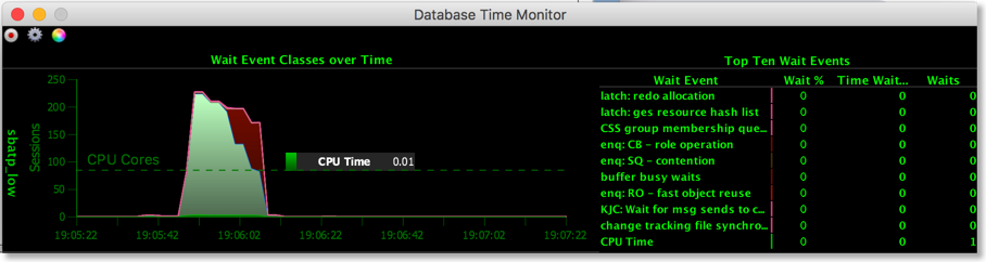
You can use this to monitor in real time the activity of the ATP instance. Currently it reports all of the cores on the server you are running on. This will be fixed shortly to just show the cores available to you.
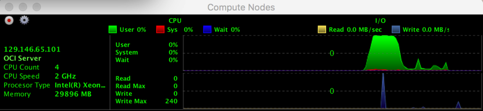
The final tool, cpumonitor (http://www.dominicgiles.com/cpumonitor.html), allows you to monitor the activity of the application server. This can be downloaded from here (http://www.dominicgiles.com/downloads.html) and again should be installed on your PC or Mac. This is done by simply unzipping the download. Then change into the bin directory on mac or linux or the winbin directory on a windows machine.
You’ll need to edit the XML file to reflect the location of the application server.
Save the file and then launch it with the command
$> ./cpumonitor
Conclusion
That's it. We’ve installed swingbench against Oracle Autonomous Transaction Processing. In my next blog entry we'll take a look at some automated tests you can user to kick the tyres on ATP. I'll also include a version that shows how to install the TPC-DS like schema that comes with swingbench against Oracle Autonomous Warehouse.
New version of Database Time Viewer
An example of connecting to ATP might be
$> ./dbtimemonitor -u admin -p
or on Windows
$> dbtimemonitor.bat -u admin -p
There's no need to uncompress the credentials file just specify the zip file.
Creating, Querying and Loading Data in to the Oracle Autonomous Data Warehouse
Oracle Autonomous Data Warehouse (ADW) access via Python
The following shows how to access the Oracle Autonomous Data Warehouse using Python and how to load the data using the DBMS_CLOUD package via the cx_Oracle module. This is obviously simpler via the Graphical front end or SQL Developer but using Python provdes a simple scriptable model whilst hiding some of the complexities of using native REST APIs.
This simple example assumes that you've got an Oracle Cloud account and that you've created or got access an ADW database. You'll also have to download the credentials file to provide SQL*Net access. You can find the details on how to do that here. We'll be using Python in this short example but most of what we're doing could be achieved using the GUI and/or REST Calls.
Connecting to ADW Instance
To start with we'll make sure we can connect to the ADW Instance we've previously created. To do that we need to import the required libraries. If you dodn't have these I reccommend using PIP (and virtualenv)
import cx_Oracle
import keyring
import os
We need to use an environment variable to reflect the location of the downloaded credentials files to be used by SQL*Net.
os.environ['TNS_ADMIN'] = '/Users/dgiles/Downloads/wallet_DOMSDB'
This is equivlent to bash
export TNS_ADMIN=/Users/dgiles/Downloads/wallet_DOMSDB and points to the unzipped directory containing the tnsnames.ora, sqlnet.ora etc. NOTE: you'll need to update the sqlnet.ora to ensure the wallet points to the same directory specified in the TNS_ADMIN environment variable. i.e.
WALLET_LOCATION = (SOURCE = (METHOD = file) (METHOD_DATA = (DIRECTORY="/Users/dgiles/Downloads/wallet_DOMSDB")))
SSL_SERVER_DN_MATCH=yes
In the example above I've changed DIRECTORY to the location where I downloaded and unzipped the credentials file.
The next steps are to connect to the Oracle ADW instance. In the example below I've store my password using the Python Module "keyring". I'm also using the jupyter notebook magic sql functionality. We'll test the connection using the admin user and the connect string "domsdb_medium" which is one of the services included in the tnsnames.ora file.
%load_ext sql
password = keyring.get_password('adw','admin')
%sql oracle+cx_oracle://admin:$password@domsdb_medium
%%sql admin@domsdb_medium
select 1 from dual
Generating test data
We've connected to the oracle database and can now start uploading data to the instance. In this example we'll use datagenerator to generate the data into flat files and then place these on Oracle Object Store and load them from there.
The first step is to install datagenerator. You can find details on how to do that here. We can now simply generate data for the "SH" benchmark.
import subprocess

# Change the 2 following parameters to reflect your environment
generated_data_dir = '/Users/dgiles/Downloads/generated_data'
datagenerator_home = '/Users/dgiles/datagenerator'

# Change the following paramters relating to the way datagenerator will create the data
scale = 100
parallel = 8

dg_command = '{dg}/bin/datagenerator -c {dg}/bin/sh.xml -scale {s} -cl -f -d {gdd} -tc {p}'.format(
    dg = datagenerator_home,
    s = scale,
    gdd = generated_data_dir,
    p = parallel
)
# Typically we'd use a command similiar to the one below but since we're in a notebook it's easier to use the default functionality
# p = subprocess.Popen(command, shell=True, stdout=subprocess.PIPE)
# (output, err) = p.communicate()

print(dg_command)
!{dg_command}
We should now have a series of files in the "generated_data_dir" directory. These will be a mix of csv files, create table scripts, loader scripts etc.
!ls {generated_data_dir}
Uploading the data to the Oracle Object Store
We're really only interested in the "csv" files so we'll upload just those. But before we do this we'll need to establish a connection to the Oracle Object Store. I give some detail behind how to do this in this notebook. I'll be using the object storage out of the Frankfurt Region.
import oci
import ast

my_config = ast.literal_eval(keyring.get_password('oci_opj','doms'))
my_config['region'] = 'eu-frankfurt-1'
object_storage_client = oci.object_storage.ObjectStorageClient(my_config)
namespace = object_storage_client.get_namespace().data
We've now got a handle to the Oracle Object Store Client so we can now create a bucket which we'll call and upload the "CSV" Files.
import os, io

bucket_name = 'Sales_Data'

files_to_process = [file for file in os.listdir(generated_data_dir) if file.endswith('csv')]

try:
    create_bucket_response = object_storage_client.create_bucket(
        namespace,
        oci.object_storage.models.CreateBucketDetails(
            name=bucket_name,
            compartment_id=my_config['tenancy']
        )
    )
except Exception as e:
    print(e.message)


for upload_file in files_to_process:
    print('Uploading file {}'.format(upload_file))
    object_storage_client.put_object(namespace, bucket_name, upload_file, io.open(os.path.join(generated_data_dir,upload_file),'r'))
We need to create an authentication token that can be used by the ADW instance to access our Object storage. To do this we need to create an identity client.
indentity_client = oci.identity.IdentityClient(my_config)
token = indentity_client.create_auth_token(
    oci.identity.models.CreateAuthTokenDetails(
        description = "Token used to provide access to newly loaded files"
    ),
    user_id = my_config['user']
)
Creating users and tables in the ADW Instance
The following steps will feel very familiar to any DBA/developer of and Oracle database. We need to create a schema and assocated tables to load the data into.
First we'll need to create a user/schema and grant it the appropriate roles
%sql create user mysh identified by ReallyLongPassw0rd default tablespace data
Grant the "mysh" user the DWROLE
%sql grant DWROLE to mysh
%sql oracle+cx_oracle://mysh:ReallyLongPassw0rd@domsdb_medium
We can now create the tables we'll use to load the data into.
%%sql mysh@domsdb_medium
CREATE TABLE COUNTRIES (
  COUNTRY_ID           NUMBER       NOT NULL,
  COUNTRY_ISO_CODE     CHAR(2)      NOT NULL,
  COUNTRY_NAME         VARCHAR2(40) NOT NULL,
  COUNTRY_SUBREGION    VARCHAR2(30) NOT NULL,
  COUNTRY_SUBREGION_ID NUMBER       NOT NULL,
  COUNTRY_REGION       VARCHAR2(20) NOT NULL,
  COUNTRY_REGION_ID    NUMBER       NOT NULL,
  COUNTRY_TOTAL        NUMBER(9)    NOT NULL,
  COUNTRY_TOTAL_ID     NUMBER       NOT NULL,
  COUNTRY_NAME_HIST    VARCHAR2(40)
)
%%sql mysh@domsdb_medium
CREATE TABLE SALES (
  PROD_ID       NUMBER     NOT NULL,
  CUST_ID       NUMBER     NOT NULL,
  TIME_ID       DATE       NOT NULL,
  CHANNEL_ID    NUMBER     NOT NULL,
  PROMO_ID      NUMBER     NOT NULL,
  QUANTITY_SOLD NUMBER(10) NOT NULL,
  AMOUNT_SOLD   NUMBER(10) NOT NULL
)
%%sql mysh@domsdb_medium
CREATE TABLE SUPPLEMENTARY_DEMOGRAPHICS (
  CUST_ID                 NUMBER NOT NULL,
  EDUCATION               VARCHAR2(21),
  OCCUPATION              VARCHAR2(21),
  HOUSEHOLD_SIZE          VARCHAR2(21),
  YRS_RESIDENCE           NUMBER,
  AFFINITY_CARD           NUMBER(10),
  BULK_PACK_DISKETTES     NUMBER(10),
  FLAT_PANEL_MONITOR      NUMBER(10),
  HOME_THEATER_PACKAGE    NUMBER(10),
  BOOKKEEPING_APPLICATION NUMBER(10),
  PRINTER_SUPPLIES        NUMBER(10),
  Y_BOX_GAMES             NUMBER(10),
  OS_DOC_SET_KANJI        NUMBER(10),
  COMMENTS                VARCHAR2(4000)
)
%%sql mysh@domsdb_medium
CREATE TABLE CUSTOMERS (
  CUST_ID                NUMBER       NOT NULL,
  CUST_FIRST_NAME        VARCHAR2(20) NOT NULL,
  CUST_LAST_NAME         VARCHAR2(40) NOT NULL,
  CUST_GENDER            CHAR(1)      NOT NULL,
  CUST_YEAR_OF_BIRTH     NUMBER(4)    NOT NULL,
  CUST_MARITAL_STATUS    VARCHAR2(20),
  CUST_STREET_ADDRESS    VARCHAR2(40) NOT NULL,
  CUST_POSTAL_CODE       VARCHAR2(10) NOT NULL,
  CUST_CITY              VARCHAR2(30) NOT NULL,
  CUST_CITY_ID           NUMBER       NOT NULL,
  CUST_STATE_PROVINCE    VARCHAR2(40) NOT NULL,
  CUST_STATE_PROVINCE_ID NUMBER       NOT NULL,
  COUNTRY_ID             NUMBER       NOT NULL,
  CUST_MAIN_PHONE_NUMBER VARCHAR2(25) NOT NULL,
  CUST_INCOME_LEVEL      VARCHAR2(30),
  CUST_CREDIT_LIMIT      NUMBER,
  CUST_EMAIL             VARCHAR2(40),
  CUST_TOTAL             VARCHAR2(14) NOT NULL,
  CUST_TOTAL_ID          NUMBER       NOT NULL,
  CUST_SRC_ID            NUMBER,
  CUST_EFF_FROM          DATE,
  CUST_EFF_TO            DATE,
  CUST_VALID             VARCHAR2(1)
)
%%sql mysh@domsdb_medium
CREATE TABLE CHANNELS (
  CHANNEL_ID       NUMBER       NOT NULL,
  CHANNEL_DESC     VARCHAR2(20) NOT NULL,
  CHANNEL_CLASS    VARCHAR2(20) NOT NULL,
  CHANNEL_CLASS_ID NUMBER       NOT NULL,
  CHANNEL_TOTAL    VARCHAR2(13) NOT NULL,
  CHANNEL_TOTAL_ID NUMBER       NOT NULL
)
%%sql mysh@domsdb_medium
CREATE TABLE PRODUCTS (
  PROD_ID               NUMBER(6)      NOT NULL,
  PROD_NAME             VARCHAR2(50)   NOT NULL,
  PROD_DESC             VARCHAR2(4000) NOT NULL,
  PROD_SUBCATEGORY      VARCHAR2(50)   NOT NULL,
  PROD_SUBCATEGORY_ID   NUMBER         NOT NULL,
  PROD_SUBCATEGORY_DESC VARCHAR2(2000) NOT NULL,
  PROD_CATEGORY         VARCHAR2(50)   NOT NULL,
  PROD_CATEGORY_ID      NUMBER         NOT NULL,
  PROD_CATEGORY_DESC    VARCHAR2(2000) NOT NULL,
  PROD_WEIGHT_CLASS     NUMBER(3)      NOT NULL,
  PROD_UNIT_OF_MEASURE  VARCHAR2(20),
  PROD_PACK_SIZE        VARCHAR2(30)   NOT NULL,
  SUPPLIER_ID           NUMBER(6)      NOT NULL,
  PROD_STATUS           VARCHAR2(20)   NOT NULL,
  PROD_LIST_PRICE       NUMBER(8)      NOT NULL,
  PROD_MIN_PRICE        NUMBER(8)      NOT NULL,
  PROD_TOTAL            VARCHAR2(13)   NOT NULL,
  PROD_TOTAL_ID         NUMBER         NOT NULL,
  PROD_SRC_ID           NUMBER,
  PROD_EFF_FROM         DATE,
  PROD_EFF_TO           DATE,
  PROD_VALID            VARCHAR2(1)
)
%%sql mysh@domsdb_medium
CREATE TABLE PROMOTIONS (
  PROMO_ID             NUMBER(6)    NOT NULL,
  PROMO_NAME           VARCHAR2(30) NOT NULL,
  PROMO_SUBCATEGORY    VARCHAR2(30) NOT NULL,
  PROMO_SUBCATEGORY_ID NUMBER       NOT NULL,
  PROMO_CATEGORY       VARCHAR2(30) NOT NULL,
  PROMO_CATEGORY_ID    NUMBER       NOT NULL,
  PROMO_COST           NUMBER(10)   NOT NULL,
  PROMO_BEGIN_DATE     DATE         NOT NULL,
  PROMO_END_DATE       DATE         NOT NULL,
  PROMO_TOTAL          VARCHAR2(15) NOT NULL,
  PROMO_TOTAL_ID       NUMBER       NOT NULL
)
%%sql mysh@domsdb_medium
CREATE TABLE times AS
SELECT udate time_id,
  TO_CHAR(udate,'Day' day_name,
  TO_CHAR(udate,'DD' day_number_in_month,
  TO_CHAR(udate,'DDD' day_number_in_year,
  TO_CHAR(udate,'YYYY' ) calendar_year,
  TO_CHAR(udate,'Q' ) calendar_quarter_number,
  TO_CHAR(udate,'MM' ) calendar_month_number,
  TO_CHAR(udate,'WW' ) calendar_week_number,
  TO_CHAR(udate,'YYYY-MM' calendar_month_desc,
  TO_CHAR(udate,'YYYY-Q' calendar_quarter_desc
FROM
  (SELECT to_date('31/12/1994','DD/MM/YYYY'+rownum udate
  FROM all_objects
  WHERE to_date('31/12/1994','DD/MM/YYYY'+rownum <= to_date( '31/12/2014','DD/MM/YYYY'
  )
day_name,
TO_CHAR(udate,'DD' day_number_in_month,
TO_CHAR(udate,'DDD' day_number_in_year,
TO_CHAR(udate,'YYYY' ) calendar_year,
TO_CHAR(udate,'Q' ) calendar_quarter_number,
TO_CHAR(udate,'MM' ) calendar_month_number,
TO_CHAR(udate,'WW' ) calendar_week_number,
TO_CHAR(udate,'YYYY-MM' calendar_month_desc,
TO_CHAR(udate,'YYYY-Q' calendar_quarter_desc
FROM
(SELECT to_date('31/12/1994','DD/MM/YYYY'+rownum udate
FROM all_objects
WHERE to_date('31/12/1994','DD/MM/YYYY'+rownum <= to_date( '31/12/2014','DD/MM/YYYY'
)
%%sql mysh@domsdb_medium
select * from tab
Copying the data from the object store
We need to add the authorisation token to the newly created schema to allow it to access the object stores files. We can't do this using the sql magic syntax we've been using till this point so we'll do it using standard cx_Oracle calls.
connection = cx_Oracle.connect('mysh', 'ReallyLongPassw0rd', 'domsdb_medium')
cursor = connection.cursor();
cursor.callproc('DBMS_CLOUD.create_credential', keywordParameters = {'credential_name':'SALES_DATA_AUTH',
                                                                    'username':'dominic.giles@oracle.com',
                                                                    'password':token.data.token})
We can access the object storage using a url of the the format
https://swiftobjectstorage.<region>.oraclecloud.com/v1/<tenancy>/<bucket name>/<object name>We can use this to dynamically generate a url for each of the objects inside of the bucket we've just created and use the DBMS_CLOUD package to copy the data into the ADW instance. The code below gets all of the names of the tables we've just created and the loops through each table copying the associated csv file into the ADW instance.
from tqdm import tqdm

format = '''{"delimiter" : ",",
          "skipheaders" : 1,
          "ignoremissingcolumns" : "true",
          "removequotes" : "true",
          "dateformat" : "DD-MON-YYYY HH24:MI:SS",
          "blankasnull" : "true"}'''

file_location = '''https://swiftobjectstorage.{region}.oraclecloud.com/v1/{tenancy}/{bucket_name}/{table_name}.csv'''
region = my_config['region']
tenancy= 'oracleonpremjava'


rs = cursor.execute("select table_name from user_tables where table_name not like 'COPY%'")
rows = rs.fetchall()
for row in tqdm(rows):
    url = file_location.format(region=region, tenancy=tenancy, bucket_name=bucket_name, table_name=row[0])
    cursor.callproc('DBMS_CLOUD.copy_data', keywordParameters= {'table_name':row[0],
                                                           'credential_name':'SALES_DATA_AUTH',
                                                           'file_uri_list':url,
                                                           'format': format
                                                           })
We can now take a look and see how many rows we've loaded into the tables
rs = cursor.execute("select table_name from user_tables where table_name not like 'COPY%'")
rows = rs.fetchall()

for row in rows:
    rs2 = cursor.execute("select count(*) from {}".format(row[0]))
    rows2 = rs2.fetchone()
    print('{tn: <35}{rc:>10,}'.format(tn=row[0],rc=rows2[0]))
It's now possible to run standard queries against the newly loaded data. No need to create anything else (indexes etc.)
%%sql mysh@domsdb_medium
SELECT channels.channel_desc,
       countries.country_iso_code,
       TO_CHAR(SUM(amount_sold), '9,999,999,999' SALES$
FROM sales, customers, times, channels, countries
WHERE sales.time_id=times.time_id
  AND sales.cust_id=customers.cust_id
  AND customers.country_id = countries.country_id
  AND sales.channel_id = channels.channel_id
  AND channels.channel_desc IN ('Tele Sales','Internet'
  AND times.calendar_year = '2006'
  AND countries.country_iso_code IN ('GB','DE','FR','DK'
GROUP BY
  ROLLUP(channels.channel_desc,countries.country_iso_code)
ORDER BY 1
Tidying up the object store and database
You can run the following steps if you want to remove all of the tables from the schema and purge the object store of files. Lets start by removing the tables. NOTE : The code below will remove all of the tables from the schema. Make sure you've not got anything in the schema that you want to keep before running it.
from tqdm import tqdm

rs = cursor.execute("select table_name from user_tables")
rows = rs.fetchall()

for row in tqdm(rows):
    rs2 = cursor.execute("drop table {} purge".format(row[0]))
And then removing the object store files and bucket
object_list = object_storage_client.list_objects(namespace, bucket_name)

for o in object_list.data.objects:
    print('Deleting object {}'.format(o.name))
    object_storage_client.delete_object(namespace, bucket_name, o.name)

print('Deleting bucket')
response = object_storage_client.delete_bucket(namespace, bucket_name)
Accessing the Oracle Object Store
OCI Object Store Examples
The following are a series of examples showing the loading of data into the Oracle Object Store. For these to work with your own data you'll need to have your own Oracle Cloud account and uploaded a key. You can find details on how to achieve this here
I'll be using the Oracle OCI Python SDK which wrappers the REST API. You can find details on the API here
Before we do anything we'll need to load the required needed Python modules.
import oci
import keyring
import ast
import os
Configuration needed to connect
I'm using the "keyring" Python module to hold the config for my connection to OCI (to avoid needlessly exposing sensitive information). It's of the form
{
    "user": "your user ocid",
    "key_file": "the path to your private key file",
    "fingerprint": "the fingerprint of your public key",
    "tenancy": "your tenancy ocid",
    "region": "the region you are working with"
}
After retrieving it from my keyring store I then need to convert it into a dictionary before using it. You can also validate the config you are using as well. Handy if this is the first time you've configured it.
my_config = ast.literal_eval(keyring.get_password('oci_opj','doms'))
oci.config.validate_config(my_config)
Create object storage client
Then I just need to retireve a Object Storage client to start working with data
object_storage_client = oci.object_storage.ObjectStorageClient(my_config)
namespace = object_storage_client.get_namespace().data
bucket_name = "doms_object_store"
Upload the contents of user directory to a bucket
I'll create a bucket and then select all of the files from a user defined directory and upload them to the newly created bucket
import os, io

directory = '/Users/dgiles/datagenerator/bin/generateddata'
files_to_process = [file for file in os.listdir(directory) if file.endswith('csv')]
Create a bucket named "Sales_Data" and give it the tenancy ocid from your config.
try:
    create_bucket_response = object_storage_client.create_bucket(
        namespace,
        oci.object_storage.models.CreateBucketDetails(
            name='Sales_Data',
            compartment_id=my_config['tenancy']
        )
    )
except Exception as e:
    print(e.message)
Then we just need to loop through the list of files in the directory specified and upload them to the newly created bucket
bucket_name = 'Sales_Data'
for upload_file in files_to_process:
    print('Uploading file {}'.format(upload_file))
    object_storage_client.put_object(namespace, bucket_name, upload_file, io.open(os.path.join(directory,upload_file),'r'))
Retrieve a list of objects in a bucket
The folowing retrieves a bucket and gets a list of objects in the bucket
bucket = object_storage_client.get_bucket(namespace, bucket_name)
object_list = object_storage_client.list_objects(namespace, bucket_name)

for o in object_list.data.objects:
    print(o.name)
Download the contents of an object
The following downloads a file from a named bucket in chunks and writes it to user defined directory on the client
# Attempt to download a file

object_name = "CUSTOMERS.csv"
destination_dir = '/Users/dgiles/Downloads'.format(object_name)
get_obj = object_storage_client.get_object(namespace, bucket_name, object_name)
with open(os.path.join(destination_dir,object_name), 'wb') as f:
    for chunk in get_obj.data.raw.stream(1024 * 1024, decode_content=False):
        f.write(chunk)
Delete a bucket
We can just as simply delete the bucket we've just created but first we'll need to delete all of the objects inside of it.
object_list = object_storage_client.list_objects(namespace, bucket_name)

for o in object_list.data.objects:
    print('Deleting object {}'.format(o.name))
    object_storage_client.delete_object(namespace, bucket_name, o.name)

print('Deleting bucket')
response = object_storage_client.delete_bucket(namespace, bucket_name)
Python, Oracle_cx, Altair and Jupyter Notebooks
Simple Oracle/Jupyter/Keyring/Altair Example
In this trivial example we'll be using Jupyter Lab to create this small notebook of Python code. We will see how easy it is to run SQL and analyze those results. The point of the exercise here isn't really the SQL we use but rather how simple it is for developers or analysts who prefer working with code rather than a full blown UI to retrieve and visualise data.
For reference I'm using Python 3.6 and Oracle Database 12c Release 2. You can find the source here
First we'll need to import the required libraries. It's likely that you won't have them installed on your server/workstation. To do that use the following pip command "pip install cx_Oracle keyring pandas altair jupyter jupyter-sql". You should have pip installed and probably be using virtualenv but if you don't I'm afraid that's beyond the scope of this example. Note whilst I'm not importing jupyter and jupyter-sql in this example they are implicitly used.
import cx_Oracle
import keyring
import pandas as pd
import altair as alt
We will be using the magic-sql functionality inside of jupyter-lab. This means we can trivially embed SQL rather than coding the cusrsors and fetches we would typically have to do if we were using straight forward cx_Oracle. This uses the "magic function" syntax" which start with "%" or "%%". First we need to load the support for SQL
%load_ext sql
Next we can connect to the local docker Oracle Database. However one thing we don't want to do with notebooks when working with server application is to disclose our passwords. I use the python module "keyring" which enables you to store the password once in a platform appropriate fashion and then recall it in code. Outside of this notebook I used the keyring command line utility and ran "keyring set local_docker system". It then prompted me for a password which I'm using here. Please be careful with passwords and code notebooks. It's possible to mistakenly serialise a password and then potentially expose it when sharing notebooks with colleagues.
password = keyring.get_password('local_docker','system')
We can then connect to the Oracle Database. In this instance I'm using the cx_Oracle Diriver and telling it to connect to a local docker database running Oracle Database 12c (12.2.0.1). Because I'm using a service I need to specify that in the connect string. I also substitute the password I fetched earlier.
%sql oracle+cx_oracle://system:$password@localhost/?service_name=soe
I'm now connected to the Oracle database as the system user. I'm simply using this user as it has access to a few more tables than a typical user would. Next I can issue a simple select statement to fetch some table metadata. the %%sql result << command retrieves the result set into the variable called result
%%sql result <<
select table_name, tablespace_name, num_rows, blocks, avg_row_len, trunc(last_analyzed)
from all_tables
where num_rows  > 0
and tablespace_name is not null
In Python a lot of tabular manipulation of data is performed using the module Pandas. It's an amazing piece of code enabling you to analyze, group, filter, join, pivot columnar data with ease. If you've not used it before I strongly reccomend you take a look. With that in mind we need to take the resultset we retrieved and convert it into a DataFrame (the base Pandas tabular structure)
result_df = result.DataFrame()
We can see a sample of that result set the the Panada's head function
result_df.head()
All very useful but what if wanted to chart how many tables were owned by each user. To do that we could of course use the charting functionlty of Pandas (and Matplotlib) but I've recently started experimenting with Altair and found it to make much more sense when define what and how to plot data. So lets just plot the count of tables on the X axis and the tablespace name on the Y axis.
alt.Chart(result_df).mark_bar().encode(
    x='count()',
    y='tablespace_name',
)

Altair makes much more sense to me as a SQL user than some of the cryptic functionality of Matplotlib. But the chart looks really dull. We can trvially tidy it up a few additonal commands
alt.Chart(result_df).mark_bar().encode(
    x=alt.Y('count()', title='Number of tables in Tablespace'),
    y=alt.Y('tablespace_name', title='Tablespace Name'),
    color='tablespace_name'
).properties(width=600, height= 150, title='Tables Overview')

Much better but Altair can do significantly more sophisticated charts than a simple bar chart. Next lets take a look at the relationship between the number of rows in a table and the blocks required to store them. It's worth noting that this won't, or at least shouldn't, produce any startling results but it's a useful plot on a near empty database that will give use something to look at. Using another simple scatter chart we get the following
alt.Chart(result_df).mark_point().encode(
    y = 'num_rows',
    x = 'blocks',
).properties(width=600)

Again it's a near empty database and so there's not much going on or at least we have a lot of very small tables and a few big ones. Lets use a logarithmic scale to spread things out a little better and take the oppertunity to brighten it up
alt.Chart(result_df).mark_point().encode(
    y = alt.Y('num_rows',scale=alt.Scale(type='log')),
    x = alt.X('blocks', scale=alt.Scale(type='log')),
    color = 'tablespace_name',
    tooltip=['table_name']
).properties(width=600)

Much better... But Altair and the libraries it uses has a another fantastic trick up its sleeve. It can make the charts interactive (zoom and pan) but also enable you to select data in one chart and have it reflected in another. To do that we use a "Selection" object and use this to filter the data in a second chart. Lets do this for the two charts we created. Note you'll need to have run this notebook "live" to see the interactive selection.
interval = alt.selection_interval()

chart1 = alt.Chart(result_df).mark_point().encode(
    y = alt.Y('num_rows',scale=alt.Scale(type='log')),
    x = alt.X('blocks', scale=alt.Scale(type='log')),
    color = 'tablespace_name',
    tooltip=['table_name']
).properties(width=600, selection=interval)

chart2 = alt.Chart(result_df).mark_bar().encode(
    x='count()',
    y='tablespace_name',
    color = 'tablespace_name'
).properties(width=600, height= 150).transform_filter(
    interval
)

chart1 & chart2

And thats it. I'll be using this framework to create a few additional examples in the coming weeks.
The following shows what you would have seen if you had been running the notebook code inside of a browser
Making the alert log just a little more readable
But what if you are only looking after one or two or just testing something out? Well the most common solution is to simply tail the alert log file.
The only issue is that it's not the most exciting thing to view, this of course could be said for any terminal based text file. But there are things you can do to make it easier to parse visually and improve your chances of catching an unexpected issue.
The approach I take is to push the alert log file through python and use the various libraries to brighten it up. It's very easy to go from this (tail -f)
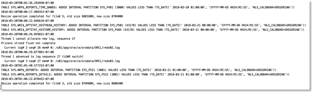
To this
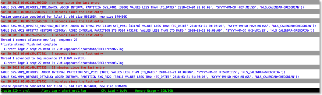
The reason this works is that python provides a rich set of libraries which can add a little bit of colour and formatting to the alert file.
You can find the code to achieve this in the gist below
Just a quick note on installing this. You'll need either python 2.7 or 3 available on your server.
I'd also recommend installing pip and then the following libraries
pip install humanize psutil colorama python-dateutil
After you've done that it's just a case of running the script. If you have $ORACLE_BASE and $ORACLE_SID set the library will try and make a guess at the location of the alert file. i.e
python alertlogparser.py
But if that doesn't work or you get an error you can also explicitly specify the location of the alert log with something like
python alertlogparser.py -a $ORACLE_BASE/diag/rdbms/orcl/orcl/trace/alert_orcl.log
This script isn't supposed to be an end product just a simple example of what can be achieved to make things a little easier. And whilst I print information like CPU load and Memory there's nothing to stop you from modifying the script to display the number of warnings or errors found in the alert log and update it things change. Or if you really want to go wild implement something similar but a lot more sophisticated using python and curses
The age of "Terminal" is far from over….
New build of swingbench... Testers needed!!
Change log
- Reverted back to the old chart engine rather than JavaFX to ensure charts now render on Linux as well as Mac and Windows
- Improvements in code to ensure that results are always written to a results file or the screen
- Charbench now has the option of producing a simple human readable report at the end of the run via the "-mr" command line option
- Users can now update the meta data at the end of a run with the sbutil utility to ensure it reflects the changes that have taken place
- Better handling of errors when attempting to start graphical utils on server without an output device to render to (headless)
As always you can download it from here