2015
Update to cpumonitor... first of many
28/09/15 15:05 Filed in: cpumonitor
I've updated cpumonitor for the first time in a while. This brings the first of many release as I gradually drag the swingbench code base up to Java 8 conformance. This build now requires Java 8. The few changes I've made are
- The record button now outputs a CSV as opposed a tab delimited file.
- Removed unnecessary output in the "micro" version
- Updated ssh libraries to latest version
Comments
Oracle, Pythons and Pandas... Oh My.
14/08/15 12:06
Over the last year I've been using Python more frequently and enjoying the experience. Some things are just simpler to do in Python than my go to language, Java. One area that makes things simpler is the extensive range of libraries and the simplicity of installing and maintaining them… This blog isn't intended to be an introduction to python and it's many libraries just a quick intro to those I seem to use more and more.
There are few libraries that are perfect for working with a database.
Also one aspect that I'm not going to cover but that really takes Python from an expressive programming language to a collaborative to a tool for sophisticated collaborative data exploration and development is IPython Notebook. IT provides a means of writing up and executing live code that can be modified by other collaborators. I'll cover this in a future blog.
Before we go any further we need to make sure we have python installed and the correct libraries. I'm using Python 2.7 but the code we are using should work fine with python 3.0. Most operating systems will have have python installed by default. If yours doesn't you can get it here. Next we need to insure that we have all of the correct libraries. To do this I use the python library manager "pip". Again I won't go into it's installation if you don't have it installed but you can find details here. After you've installed pip all you need to do to ensure you've got the correct libraries is to issue a command like
This will sort out all the dependencies for you. I've also used the "—upgrade" option to ensure we refresh any out of date libraries. If you get permission errors it's likey to be because you don't have the privilege to install the libraries into the shared system lib location. Either rerun the command as root or with sudo i.e.
Or create a virtual environment
You can check to see that your libraries are installed by using the "pip list" command.
For the impatient amongst you lets start with code and explain some of the details later
On running the code with a command like. Note : I saved my code to a file dbtime60min.py
You should see a chart like the following.
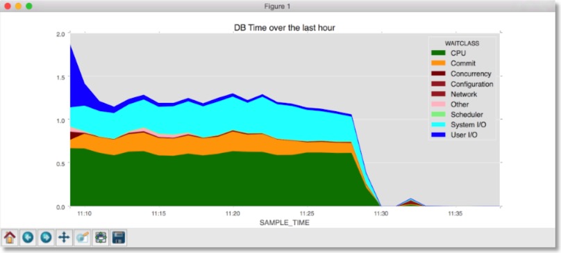
So in a relatively short amount of code we can quickly produce a useful chart. And the beauty of the solution is that we could replace the relatively complex piece of SQL I used with some thing more trivial and Pandas does much of the heavy lifting to convert it into a useful chart that we can share with others.
There are a view areas that are worth understanding in the code and that highlight the easy of working with a a framework like Pandas.
I created a function "def read_from_db" that connects to the database (via the cx_oracle library) and then asks the Pandas framework to read the data back from the database.
The Pandas reads this data into a multi dimensional structure, much like the table we read this information from. And just like a database table Pandas enables us to sort and filter the data. Using a command like
Shows us the details of the information we've just read in. i.e.
We can also see a sample of the data with "tail()" or "head()" i.e.
results in
We can also select individual columns from this data set with a command like
Which will give us
Instead of explicitly iterating through the data to find information we can also filter out just the relevant information i.e.
Which will enable us to just select data from the dataset where the WAITCLASS column only contains 'CPU. Very similar to a SQL where clause i.e. "where WAITCLASS = 'CPU'. When we print the head of the fdf Data frame we get
Another capability of Pandas (and there are many and we've only touched on a few) is the ability to pivot the data. Now in this example you could make the case it would have been simpler to pivot the data in the database. But I'm doing it here to illustrate the point. All we need to do is to specify which columns will be the index (y axis) and which column(s) will be the column headers (x axis) and which column will be the value.
will turn this time series data
into this pivoted data
The last step is to chart the data and this is achieved in a single command in Pandas.
There's a couple of things to note. I've overwritten the default colour map to use colours that would be familiar to Oracle DBAs via the Enterprise Managers DB Time charts. And I also didn't use a colour map to ensure that CPU is always rendered in "green".
So just a quick example of the power of Pandas when used in conjunction with Oracle. I'll try and post a few more Python articles over the coming weeks.
There are few libraries that are perfect for working with a database.
- cx_oracle : This driver enables you to connect to the oracle database via Oracle's OCI Client. You'll need to install Oracle's instant or full client.
- MatPlotLib : A powerful charting library enabling you to visualise your data in an unimaginalable number of ways
- Pandas : An easy to use library for data analysis
- Numpy : A powerful scientific computing package
Also one aspect that I'm not going to cover but that really takes Python from an expressive programming language to a collaborative to a tool for sophisticated collaborative data exploration and development is IPython Notebook. IT provides a means of writing up and executing live code that can be modified by other collaborators. I'll cover this in a future blog.
Setting up Python
Before we go any further we need to make sure we have python installed and the correct libraries. I'm using Python 2.7 but the code we are using should work fine with python 3.0. Most operating systems will have have python installed by default. If yours doesn't you can get it here. Next we need to insure that we have all of the correct libraries. To do this I use the python library manager "pip". Again I won't go into it's installation if you don't have it installed but you can find details here. After you've installed pip all you need to do to ensure you've got the correct libraries is to issue a command like
pip install matplotlib numpy cx_oracle pandas --upgrade
This will sort out all the dependencies for you. I've also used the "—upgrade" option to ensure we refresh any out of date libraries. If you get permission errors it's likey to be because you don't have the privilege to install the libraries into the shared system lib location. Either rerun the command as root or with sudo i.e.
sudo pip install matplotlib numpy cx_oracle pandas --upgrade
Or create a virtual environment
You can check to see that your libraries are installed by using the "pip list" command.
Code
For the impatient amongst you lets start with code and explain some of the details later
__author__ = 'dgiles'

import cx_Oracle
import pandas as pd
import matplotlib.pyplot as plt
from matplotlib import style

def read_from_db (username, password, connectString, mode=None, save=False):

    if mode is None:
        connection = cx_Oracle.connect(username, password, connectString)
    else:
        connection = cx_Oracle.connect(username, password, connectString, mode)
    with connection:
        try:
            df = pd.read_sql_query("SELECT\
                                      wc.wait_class                    AS waitclass,\
                                      TRUNC(begin_time, 'MI')          AS sample_time,\
                                      round((wh.time_waited) / wh.intsize_csec, 3) AS DB_time\
                                    FROM V$SYSTEM_WAIT_CLASS wc,\
                                      v$waitclassmetric_history wh\
                                    WHERE wc.wait_class != 'Idle'\
                                          AND wc.wait_class_id = wh.wait_class_id\
                                    UNION\
                                    SELECT\
                                      'CPU'                   AS waitclass,\
                                      TRUNC(begin_time, 'MI') AS sample_time,\
                                      round(VALUE/100, 3)         AS DB_time\
                                    FROM v$sysmetric_history\
                                    WHERE GROUP_ID = 2\
                                          AND metric_name = 'CPU Usage Per Sec'\
                                    ORDER by sample_time, waitclass",
                                   connection)
            if save:
                df.to_csv('results.csv')
            return df
        except cx_Oracle.DatabaseError as dberror:
            print dberror

def read_from_file(filename):
    return pd.read_csv(filename, parse_dates=['SAMPLE_TIME'])


if __name__ == '__main__':
    style.use('ggplot')
    df = read_from_db(username='sys', password='welcome1', connectString='oracle12c2/soe', mode=cx_Oracle.SYSDBA, save=True)
    # df = read_from_file('results.csv')

    print df.head()

    pdf = df.pivot(index='SAMPLE_TIME', columns='WAITCLASS', values='DB_TIME')

    print pdf.head()

    pdf.plot(kind='area', stacked=True, title='DB Time over the last hour', color=['red', 'green', 'orange', 'darkred', 'brown', 'brown', 'pink', 'lightgreen', 'cyan', 'blue'])
    plt.show()
On running the code with a command like. Note : I saved my code to a file dbtime60min.py
python dbtime60min.py
You should see a chart like the following.
So in a relatively short amount of code we can quickly produce a useful chart. And the beauty of the solution is that we could replace the relatively complex piece of SQL I used with some thing more trivial and Pandas does much of the heavy lifting to convert it into a useful chart that we can share with others.
An explanation of the code
There are a view areas that are worth understanding in the code and that highlight the easy of working with a a framework like Pandas.
I created a function "def read_from_db" that connects to the database (via the cx_oracle library) and then asks the Pandas framework to read the data back from the database.
df = pd.read_sql_query("SELECT\
                      wc.wait_class                    AS waitclass,\
                      TRUNC(begin_time, 'MI')          AS sample_time,\
                      round((wh.time_waited) / wh.intsize_csec, 3) AS DB_time\
                    FROM V$SYSTEM_WAIT_CLASS wc,\
                      v$waitclassmetric_history wh\
                    WHERE wc.wait_class != 'Idle'\
                          AND wc.wait_class_id = wh.wait_class_id\
                    UNION\
                    SELECT\
                      'CPU'                   AS waitclass,\
                      TRUNC(begin_time, 'MI') AS sample_time,\
                      round(VALUE/100, 3)         AS DB_time\
                    FROM v$sysmetric_history\
                    WHERE GROUP_ID = 2\
                          AND metric_name = 'CPU Usage Per Sec'\
                    ORDER by sample_time, waitclass",
                   connection)
The Pandas reads this data into a multi dimensional structure, much like the table we read this information from. And just like a database table Pandas enables us to sort and filter the data. Using a command like
print.info()
Shows us the details of the information we've just read in. i.e.
Int64Index: 549 entries, 0 to 548
Data columns (total 3 columns):
WAITCLASS      549 non-null object
SAMPLE_TIME    549 non-null datetime64[ns]
DB_TIME        549 non-null float64
dtypes: datetime64[ns](1), float64(1), object(1)
memory usage: 17.2+ KB
We can also see a sample of the data with "tail()" or "head()" i.e.
print.head()
results in
       WAITCLASS         SAMPLE_TIME  DB_TIME
0            CPU 2015-08-17 11:47:00        0
1         Commit 2015-08-17 11:47:00        0
2    Concurrency 2015-08-17 11:47:00        0
3  Configuration 2015-08-17 11:47:00        0
4        Network 2015-08-17 11:47:00        0
We can also select individual columns from this data set with a command like
wcdf = df['WAITCLASS']
print wcdf.head()
Which will give us
0              CPU
1           Commit
2      Concurrency
3    Configuration
4          Network
Instead of explicitly iterating through the data to find information we can also filter out just the relevant information i.e.
fdf = df[df['WAITCLASS'] == 'CPU']
Which will enable us to just select data from the dataset where the WAITCLASS column only contains 'CPU. Very similar to a SQL where clause i.e. "where WAITCLASS = 'CPU'. When we print the head of the fdf Data frame we get
print fdf.head()
  WAITCLASS         SAMPLE_TIME  DB_TIME
0        CPU 2015-08-17 12:38:00    0.001
9        CPU 2015-08-17 12:39:00    0.001
18       CPU 2015-08-17 12:40:00    0.000
27       CPU 2015-08-17 12:41:00    0.003
36       CPU 2015-08-17 12:42:00    0.000
Another capability of Pandas (and there are many and we've only touched on a few) is the ability to pivot the data. Now in this example you could make the case it would have been simpler to pivot the data in the database. But I'm doing it here to illustrate the point. All we need to do is to specify which columns will be the index (y axis) and which column(s) will be the column headers (x axis) and which column will be the value.
pdf = df.pivot(index='SAMPLE_TIME', columns='WAITCLASS', values='DB_TIME')
will turn this time series data
       WAITCLASS         SAMPLE_TIME  DB_TIME
0            CPU 2015-08-17 12:47:00        0
1         Commit 2015-08-17 12:47:00        0
2    Concurrency 2015-08-17 12:47:00        0
3  Configuration 2015-08-17 12:47:00        0
4        Network 2015-08-17 12:47:00        0
into this pivoted data
WAITCLASS              CPU  Commit  Concurrency  Configuration  Network  \
SAMPLE_TIME
2015-08-17 12:47:00  0.000       0            0              0        0
2015-08-17 12:48:00  0.002       0            0              0        0
2015-08-17 12:49:00  0.001       0            0              0        0
2015-08-17 12:50:00  0.000       0            0              0        0
2015-08-17 12:51:00  0.000       0            0              0        0

WAITCLASS            Other  Scheduler  System I/O  User I/O
SAMPLE_TIME
2015-08-17 12:47:00  0.000          0           0         0
2015-08-17 12:48:00  0.001          0           0         0
2015-08-17 12:49:00  0.002          0           0         0
2015-08-17 12:50:00  0.000          0           0         0
2015-08-17 12:51:00  0.000          0           0         0
The last step is to chart the data and this is achieved in a single command in Pandas.
pdf.plot(kind='area', stacked=True, title='DB Time over the last hour', color=['red', 'green', 'orange', 'darkred', 'brown', 'brown', 'pink', 'lightgreen', 'cyan', 'blue'])
plt.show()
There's a couple of things to note. I've overwritten the default colour map to use colours that would be familiar to Oracle DBAs via the Enterprise Managers DB Time charts. And I also didn't use a colour map to ensure that CPU is always rendered in "green".
So just a quick example of the power of Pandas when used in conjunction with Oracle. I'll try and post a few more Python articles over the coming weeks.
Upgrade to Rapid Weaver 6.0
16/07/15 09:44
I've just upgraded to RapidWeaver 6.0 and may have broken a whole ton of links and formatting on the website. I needed to do this to enable me to reliably update content. If it all holds together over the coming weeks I'll being to change the look and feel of the site and update some of the existing content to better reflect recent changes to the swingbench family of tools.
Thanks for you patience
Dom
Thanks for you patience
Dom
SBUtil in Action (And Some Fixes)
12/03/15 18:44 Filed in: Swingbench
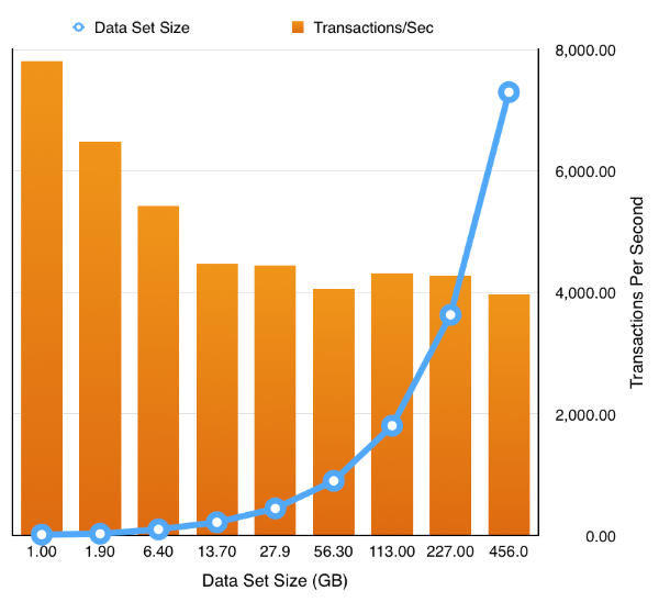
As a means of demonstrating what you can achieve with SBUtil I’ve created a little test to show it’s possible to trivially change the size of the data set and rerun the same workload to show how TPS can vary if the SGA/Buffer Cache is kept consistent.
First the script
I’m hoping it should be fairly obvious what the script does. I create a tablespace big enough to accommodate the final data set (In this instance 1TB). This way I’m not constantly auto extending the tablespace. Then I create a seed schema at 1GB in size. Then I run a workload against the schema, this will remain constant through all of the tests. Each of the load tests runs for 10min and collects full stats. After the test has completed I use “sbutil” to replicate the schema and simply rerun the workload writing the results to a new file. By the end of the tests and duplication the end schema has roughly ½ a Terabytes worth of data and about the same in indexes. The benefit of this approach is that it’s much quicker to expand the data than using the wizard to do it.
The directory will now contain all of the results files which can be processed trivially using the the “parse_results.py” script in utils directory. In the example below I simply parse all of the files and write the result to a file called res1.csv. Because the python script is so easy to modify you could pull out any of the stats from the file. I’m just using the ones that it collects by default
On completing this step I can use my favourite spread sheet tool to load res1.csv and take a look at the data. In this instance I’m using “Numbers” on OS X but Excel would work equally as well.
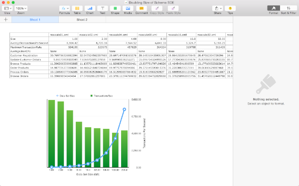
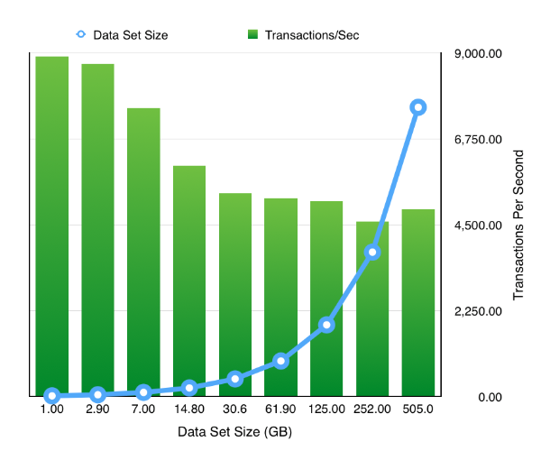
The resulting chart shows pretty much what we’d expect .That doubling the size of the datasets but keeping the workload and SGA constant results in a reduction of the TPS. Which tails off quickly as the data set quickly outgrows the buffer cache and we are forced to perform physical IOs, but declines less slowly after this impact is felt. It’s something we would expect but it’s nice to able to demonstrate it.
So the next obvious question is how easy is it to rerun the test but to enable a feature like partitioning. Really easy. Simply ask oewizard to create the schema using hash partitioning i.e. change
to
and rerun the tests to produce the following results
Or even enabling compression and partitioning by simply replacing the first sbutil operation with
During the testing of this I fixed up a few bugs which I wasn’t aware of so it’s worth downloading a new build which you can find here. I also released I needed a few more options on the utility to round it out. These were
I’ll most likely add a few more over the coming weeks.
Just a word of caution… I’ve noticed that my stats collection is broken. I don’t cater for all of the possible version/configurations in my script and so it can break on large stats collections and go serial. I’ll try and fix this next week.
First the script
#!/bin/bash

sqlplus sys/welcome1@//ed2xcomp01/DOMS as sysdba << EOF
create bigfile tablespace SOE datafile size 1000G;
exit;
EOF

time ./oewizard -scale 1 -dbap welcome1 -u soe -p soe -cl -cs //ed2xcomp01/DOMS -ts SOE -create

time ./charbench -u soe -p soe -cs //ed2xcomp01/DOMS -uc 128 -min -0 -max 0 -stats full -rt 0:10 -bs 0:01 -a -r resscale01.xml

time ./sbutil -u soe -p soe -cs //ed2xcomp01/DOMS -soe -parallel 64 -dup 2

time ./charbench -u soe -p soe -cs //ed2xcomp01/DOMS -uc 128 -min -0 -max 0 -stats full -rt 0:10 -bs 0:01 -a -r resscale02.xml

time ./sbutil -u soe -p soe -cs //ed2xcomp01/DOMS -soe -parallel 64 -dup 2

time ./charbench -u soe -p soe -cs //ed2xcomp01/DOMS -uc 128 -min -0 -max 0 -stats full -rt 0:10 -bs 0:01 -a -r resscale04.xml

time ./sbutil -u soe -p soe -cs //ed2xcomp01/DOMS -soe -parallel 64 -dup 2

time ./charbench -u soe -p soe -cs //ed2xcomp01/DOMS -uc 128 -min -0 -max 0 -stats full -rt 0:10 -bs 0:01 -a -r resscale08.xml

time ./sbutil -u soe -p soe -cs //ed2xcomp01/DOMS -soe -parallel 64 -dup 2

time ./charbench -u soe -p soe -cs //ed2xcomp01/DOMS -uc 128 -min -0 -max 0 -stats full -rt 0:10 -bs 0:01 -a -r resscale16.xml

time ./sbutil -u soe -p soe -cs //ed2xcomp01/DOMS -soe -parallel 64 -dup 2

time ./charbench -u soe -p soe -cs //ed2xcomp01/DOMS -uc 128 -min -0 -max 0 -stats full -rt 0:10 -bs 0:01 -a -r resscale32.xml

time ./sbutil -u soe -p soe -cs //ed2xcomp01/DOMS -soe -parallel 64 -dup 2

time ./charbench -u soe -p soe -cs //ed2xcomp01/DOMS -uc 128 -min -0 -max 0 -stats full -rt 0:10 -bs 0:01 -a -r resscale64.xml

time ./sbutil -u soe -p soe -cs //ed2xcomp01/DOMS -soe -parallel 64 -dup 2

time ./charbench -u soe -p soe -cs //ed2xcomp01/DOMS -uc 128 -min -0 -max 0 -stats full -rt 0:10 -bs 0:01 -a -r resscale128.xml

time ./sbutil -u soe -p soe -cs //ed2xcomp01/DOMS -soe -parallel 64 -dup 2

time ./charbench -u soe -p soe -cs //ed2xcomp01/DOMS -uc 128 -min -0 -max 0 -stats full -rt 0:10 -bs 0:01 -a -r resscale256.xml
I’m hoping it should be fairly obvious what the script does. I create a tablespace big enough to accommodate the final data set (In this instance 1TB). This way I’m not constantly auto extending the tablespace. Then I create a seed schema at 1GB in size. Then I run a workload against the schema, this will remain constant through all of the tests. Each of the load tests runs for 10min and collects full stats. After the test has completed I use “sbutil” to replicate the schema and simply rerun the workload writing the results to a new file. By the end of the tests and duplication the end schema has roughly ½ a Terabytes worth of data and about the same in indexes. The benefit of this approach is that it’s much quicker to expand the data than using the wizard to do it.
The directory will now contain all of the results files which can be processed trivially using the the “parse_results.py” script in utils directory. In the example below I simply parse all of the files and write the result to a file called res1.csv. Because the python script is so easy to modify you could pull out any of the stats from the file. I’m just using the ones that it collects by default
$ python ../utils/parse_results.py -r resscale01.xml resscale02.xml resscale04.xml resscale08.xml resscale16.xml resscale32.xml resscale64.xml resscale9128.xml resscale9256.xml -o res1.csv
On completing this step I can use my favourite spread sheet tool to load res1.csv and take a look at the data. In this instance I’m using “Numbers” on OS X but Excel would work equally as well.
The resulting chart shows pretty much what we’d expect .That doubling the size of the datasets but keeping the workload and SGA constant results in a reduction of the TPS. Which tails off quickly as the data set quickly outgrows the buffer cache and we are forced to perform physical IOs, but declines less slowly after this impact is felt. It’s something we would expect but it’s nice to able to demonstrate it.
So the next obvious question is how easy is it to rerun the test but to enable a feature like partitioning. Really easy. Simply ask oewizard to create the schema using hash partitioning i.e. change
time ./oewizard -scale 1 -dbap welcome1 -u soe -p soe -cl -cs //ed2xcomp01/DOMS -ts SOE -create
to
time ./oewizard -scale 1 -hashpart -dbap welcome1 -u soe -p soe -cl -cs //ed2xcomp01/DOMS -ts SOE -create
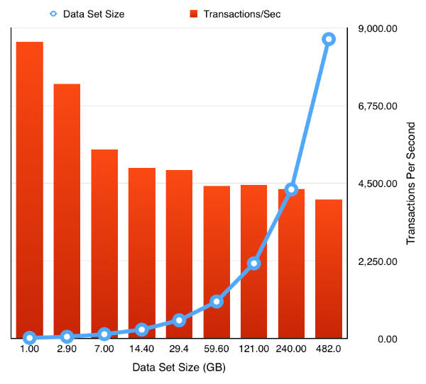
and rerun the tests to produce the following results
Or even enabling compression and partitioning by simply replacing the first sbutil operation with
time ./sbutil -u soe -p soe -cs //ed2xcomp01/DOMS -soe -parallel 64 -dup 2 -ac
During the testing of this I fixed up a few bugs which I wasn’t aware of so it’s worth downloading a new build which you can find here. I also released I needed a few more options on the utility to round it out. These were
- “seqs” : this recreates the sequences used by the schemas
- “code” : rebuilds any stored procedures
I’ll most likely add a few more over the coming weeks.
Just a word of caution… I’ve noticed that my stats collection is broken. I don’t cater for all of the possible version/configurations in my script and so it can break on large stats collections and go serial. I’ll try and fix this next week.
Swingbench Util... Going Big...
07/03/15 16:55 Filed in: Swingbench
I’ve added a utility to swingbench that perhaps I should’ve done a long time ago. The idea behind it is that it enables you to validate, fix or duplicate the data created by the wizards. I’m often contacted by people asking me how to fix an install of “Order Entry” or the “Sales History” benchmark after they’ve been running for many hours only to find they run out of temp space for the index creation. I’m also asked how they can make a really big “Sales History” schema when they only have relatively limited compute power and to create a multi terabyte data set might take days. Well the good news is that now, most of this should be relatively easy. The solution is a little program called “subtil” and you can find it in your bin or win bin directory.
Currently sbutil is command line only and requires a number of parameters to get it to do anything useful. The main parameters are
will duplicate the data in the soe schema but will first sort the seed data. You should see output similar to this
The following example validates a schema to ensure that the tables and indexes inside a schema are all present and valid
The output of the command will look similar to to this
The next command lists the tables in a schema
To drop the indexes in a schema use the following command
To recreate the indexes in a schema use the following command
You can download the new version of the software here.
Currently sbutil is command line only and requires a number of parameters to get it to do anything useful. The main parameters are
- “-dup” indicates the number of times you want data to be duplicated within the schema. Valid values are 1 to n. Data is copied and new primary keys/foreign keys generated where necessary. It’s recommended that you first increase/extend the tablespace before beginning the duplication. The duplication process will also rebuild the indexes and update the metadata table unless you specifically ask it not to with the “-nic” option. This is useful if you know you’ll be reduplicated the data again at a later stage.
- “-val” validates the tables and indexes in the specified schema. It will list any missing indexes or invalid code.
- “-stats” will create/recreate statistics for the indicated schema
- “-delstats” will delete all of the statistics for the indicated schema
- “-tables” will list all of the tables and row counts (based on database statistics) for the indicated schema
- “-di” will drop all of the indexes for the indicated schema
- “-ci” will recreate all of the indexes for the indicated schema
- “-u” : required. the username of the schema
- “-p” : required. the password of the schema
- “-cs” : required. the connect string of the schema. Some examples might be “localhost:1521:db12c”, “//oracleserver/soe” “//linuxserver:1526/orcl” etc.
- “-parallel” the level of parallelism to use to perform operations. Valid values are 1 to n.
- “-sort” sort the seed data before duplicating it.
- “-nic” don’t create indexes or constraints at the end of a duplication
- “-ac” convert the “main” tables to advanced compression
- “-hcc” convert the main tables to Hybrid Columnar Compression
- “-soe” : required. the target schema will be “Order Entry”
- “-sh” : required. the target schema will be “Sales History”
sbutil -u soe -p soe -cs //oracleserver/soe -dup 2 -parallel 32 -sort -soe
will duplicate the data in the soe schema but will first sort the seed data. You should see output similar to this
Getting table Info
Got table information. Completed in : 0:00:26.927
Dropping Indexes
Dropped Indexes. Completed in : 0:00:05.198
Creating copies of tables
Created copies of tables. Completed in : 0:00:00.452
Begining data duplication
Completed Iteration 2. Completed in : 0:00:32.138
Creating  Constraints
Created  Constraints. Completed in : 0:04:39.056
Creating  Indexes
Created  Indexes. Completed in : 0:02:52.198
Updating Metadata and Recompiling Code
Updated Metadata. Completed in : 0:00:02.032
Determining New Row Counts
Got New Row Counts. Completed in : 0:00:05.606
Completed Data Duplication in 0 hour(s) 9 minute(s) 44 second(s) 964 millisecond(s)
----------------------------------------------------------------------------------------------------------
|Table Name          |  Original Row Count|       Original Size|       New Row Count|            New Size|
----------------------------------------------------------------------------------------------------------
|ORDER_ITEMS         |         172,605,912|             11.7 GB|         345,211,824|             23.2 GB|
|CUSTOMERS           |          40,149,958|              5.5 GB|          80,299,916|             10.9 GB|
|CARD_DETAILS        |          60,149,958|              3.4 GB|         120,299,916|              6.8 GB|
|ORDERS              |          57,587,049|              6.7 GB|         115,174,098|             13.3 GB|
|ADDRESSES           |          60,174,782|              5.7 GB|         120,349,564|             11.4 GB|
----------------------------------------------------------------------------------------------------------
The following example validates a schema to ensure that the tables and indexes inside a schema are all present and valid
./sbutil -u soe -p soe -cs //ed2xcomp01/DOMS -soe -val
The output of the command will look similar to to this
The Order Entry Schema appears to be valid.

--------------------------------------------------
|Object Type    |     Valid|   Invalid|   Missing|
--------------------------------------------------
|Table          |        10|         0|         0|
|Index          |        26|         0|         0|
|Sequence       |         5|         0|         0|
|View           |         2|         0|         0|
|Code           |         1|         0|         0|
--------------------------------------------------
The next command lists the tables in a schema
./sbutil -u soe -p soe -cs //ed2xcomp01/DOMS -soe -tables

Order Entry Schemas Tables
----------------------------------------------------------------------------------------------------------------------
|Table Name                  |                Rows|              Blocks|           Size|   Compressed?|  Partitioned?|
----------------------------------------------------------------------------------------------------------------------
|ORDER_ITEMS                 |          17,157,056|             152,488|         11.6GB|              |           Yes|
|ORDERS                      |           5,719,160|              87,691|          6.7GB|              |           Yes|
|ADDRESSES                   |           6,000,000|              75,229|          5.7GB|              |           Yes|
|CUSTOMERS                   |           4,000,000|              72,637|          5.5GB|              |           Yes|
|CARD_DETAILS                |           6,000,000|              44,960|          3.4GB|              |           Yes|
|LOGON                       |                   0|                   0|        101.0MB|              |           Yes|
|INVENTORIES                 |                   0|                   0|         87.0MB|      Disabled|            No|
|PRODUCT_DESCRIPTIONS        |                   0|                   0|         1024KB|      Disabled|            No|
|WAREHOUSES                  |                   0|                   0|         1024KB|      Disabled|            No|
|PRODUCT_INFORMATION         |                   0|                   0|         1024KB|      Disabled|            No|
|ORDERENTRY_METADATA         |                   0|                   0|         1024KB|      Disabled|            No|
----------------------------------------------------------------------------------------------------------------------
To drop the indexes in a schema use the following command
./sbutil -u sh -p sh -cs //oracle12c2/soe -sh -di
Dropping Indexes
Dropped Indexes. Completed in : 0:00:00.925
To recreate the indexes in a schema use the following command
./sbutil -u sh -p sh -cs //oracle12c2/soe -sh -ci
Creating Partitioned Indexes and Constraints
Created  Indexes and Constraints. Completed in : 0:00:03.395
You can download the new version of the software here.
Java Version Performance
19/02/15 13:50 Filed in: Python
Sometimes it’s easy to loose track of the various version numbers for software as they continue their march ever onwards. However as I continue my plans to migrate onto Java8 and all of the coding goodness that lies within I thought it was a sensible to check what difference it would make to swingbench in terms of performance.
Now before we go any further it’s worth pointing out this was a trivial test and my results might not be representative of what you or anyone else might find.
My environment was
iMac (Retina 5K, 27-inch, Late 2014), 4 GHz Intel Core i7, 32 GB 1600 MHz DDR3 with a 500GB SSD
Oracle Database 12c (12.1.0.2) with the January Patch Bundle running in a VM with 8GB of memory.
The test is pretty simple but might have an impact on your choice of JVM when generating a lot of data (TB+) with swingbench. I simply created a 1GB SOE with the oewizard. This is a pretty CPU intensive operation for the entire stack : swingbench, the jdbc drivers and the database. The part of the operation that should be most effected by the performance of the JVM is the “Data Generation Step”.
So enough talk what impact did the JVM version have?
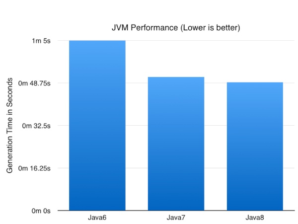
Now the numbers might not be earth shattering but it’s nice to know a simple upgrade of the JVM can result in nearly a 25% improvement in performance of a CPU/database intensive batch job. I expect these numbers to go up as I optimise some of the logic to take advantage of Java8 specific functionality.
Now before we go any further it’s worth pointing out this was a trivial test and my results might not be representative of what you or anyone else might find.
My environment was
iMac (Retina 5K, 27-inch, Late 2014), 4 GHz Intel Core i7, 32 GB 1600 MHz DDR3 with a 500GB SSD
Oracle Database 12c (12.1.0.2) with the January Patch Bundle running in a VM with 8GB of memory.
The test is pretty simple but might have an impact on your choice of JVM when generating a lot of data (TB+) with swingbench. I simply created a 1GB SOE with the oewizard. This is a pretty CPU intensive operation for the entire stack : swingbench, the jdbc drivers and the database. The part of the operation that should be most effected by the performance of the JVM is the “Data Generation Step”.
So enough talk what impact did the JVM version have?
Now the numbers might not be earth shattering but it’s nice to know a simple upgrade of the JVM can result in nearly a 25% improvement in performance of a CPU/database intensive batch job. I expect these numbers to go up as I optimise some of the logic to take advantage of Java8 specific functionality.
And now a fix to the fixes...
16/01/15 18:36 Filed in: Swingbench
Fixes to swingbench
14/01/15 12:01 Filed in: Swingbench
Happy new year….
I’ve updated swingbench with some fixes. Most of these are to do with the new results to pdf functionality. But at this point I’m giving fair warning that the following releases will be available on Java 8 only.
I’m also removing the “3d” charts from swingbench and replacing them with a richer selection of charts build using JavaFX.
Also I’ve added some simple code to the jar file to tell you which version it is… You can run this with the command
As always you can download it here. Please leave comments below if you run into any problems.
I’ve updated swingbench with some fixes. Most of these are to do with the new results to pdf functionality. But at this point I’m giving fair warning that the following releases will be available on Java 8 only.
I’m also removing the “3d” charts from swingbench and replacing them with a richer selection of charts build using JavaFX.
Also I’ve added some simple code to the jar file to tell you which version it is… You can run this with the command
$ java -jar swingbench.jar
Swingbench Version 2.5.955
As always you can download it here. Please leave comments below if you run into any problems.