Jupyter, Python, Oracle and Docker Part 3
Create Oracle Database in a Docker Container
These Python (3.6) scripts walk through the creation of a database and standby server. The reason I've done this rather than just take the default configuration is that this approach gives me a lot more control over the build and enables me to change specifc steps. If you are just wanting to get the Oracle Database running inside of Docker I strongly suggest that you use the docker files and guides in the Oracle Github repository. The approach documented below is very much for someone who is interested in a high level of control over the various steps in the installation and configuration of the Oracle Database. This current version is build on top of Oracle's Internal GiaaS docker image but will be extended to support the public dockers images as well. It aims to build an Active Data Guard model with maximum performance but can be trivially changed to support any of the required models.
It uses a mix of calls to the Docker Python API and Calls direct to the databases via cx_Oracle.
The following code section imports the needed modules to setup up our Docker container to create the Oracle Database. After that we get a Docker client handle which enables use to call the API against our local Docker environment.
import docker
import humanize
import os
import tarfile
from prettytable import PrettyTable
import cx_Oracle
from IPython.display import HTML, display
import keyring
from ipynb.fs.full.OracleDockerDatabaseFunctions import list_images,list_containers,copy_to,create_and_run_script,containter_exec,containter_root_exec,copy_string_to_file

client = docker.from_env(timeout=600)
list_images(client)
Configuration Parameters
The following section contains the parameters for setting the configuration of the install. The following parameters image_name,host_oradata,sb_host_oradata need to be changed, although sb_host_oradata is only important if you are planning on installing a standby database.
# The following parameters are specific to your install and almost certainly need to be changed
image_name = 'cc75a47617' # Taken from the id value above
host_oradata = '/Users/dgiles/Downloads/dockerdbs/oradataprimary' # The directory on the host where primary database will be persisted
sb_host_oradata = '/Users/dgiles/Downloads/dockerdbs/oradatastby' # The direcotry on the host where the standby database will be persisted
#
# The rest are fairly generic and can be changed if needed
oracle_version = '18.0.0'
db_name = 'ORCL'
stby_name = 'ORCL_STBY'
sys_password =  keyring.get_password('docker','sys') # I'm just using keyring to hide my password but you can set it to a simple sting i.e. 'mypassword'
pdb_name = 'soe'
p_host_name = 'oracleprimary'
sb_host_name = 'oraclestby'
total_memory = 2048

container_oradata = '/u01/app/oracle/oradata'
o_base = '/u01/app/oracle'
r_area = f'{o_base}/oradata/recovery_area'
o_area = f'{o_base}/oradata/'
a_area = f'{o_base}/admin/ORCL/adump'
o_home = f'{o_base}/product/{oracle_version}/dbhome_1'
t_admin = f'{o_base}/oradata/dbconfig'
log_size = 200
Create Primary Database
This code does the heavy lifting. It creates a container oracleprimary (unless you changed the paramter) running the Oracle Database. The containers 1521 port is mapped onto the the hosts 1521 port. This means that to connect from the host, via a tool like sqlplus, all you'd need to do is sqlplus soe/soe@//locahost/soe.
path = f'{o_home}/bin:/usr/local/sbin:/usr/local/bin:/usr/sbin:/usr/bin:/sbin:/bin'

p_container = client.containers.create(image_name,
                                       command="/bin/bash",
                                       hostname=p_host_name,
                                       tty=True,
                                       stdin_open=True,
                                       auto_remove=False,
                                       name=p_host_name,
                                       shm_size='3G',
                                       # network_mode='host',
                                       ports={1521:1521,5500:5500},
                                       volumes={host_oradata: {'bind': container_oradata, 'mode': 'rw'}},
                                       environment={'PATH':path,'ORACLE_SID': db_name, 'ORACLE_BASE': o_base,'TNS_ADMIN': t_admin}
                                       )

p_container.start()
# Make all of the containers attributes available via Python Docker API
p_container.reload()
The next step uses DBCA and configures features like Automatic Memory Mangement, Oracle Managed Files and sets the size of the SGA and redo logs. It prints out the status of the creation during it's progression. NOTE : This step typically takes 10 to 12 minutes.
statement = f'''dbca -silent \
 -createDatabase \
 -templateName General_Purpose.dbc \
 -gdbname {db_name} -sid {db_name} -responseFile NO_VALUE \
 -characterSet AL32UTF8 \
 -sysPassword {sys_password} \
 -systemPassword {sys_password} \
 -createAsContainerDatabase true \
 -numberOfPDBs 1 \
 -pdbName {pdb_name} \
 -pdbAdminPassword {sys_password} \
 -databaseType MULTIPURPOSE \
 -totalMemory {total_memory} \
 -memoryMgmtType AUTO_SGA \
 -recoveryAreaDestination "{r_area}" \
 -storageType FS \
 -useOMF true \
 -datafileDestination "{o_area}" \
 -redoLogFileSize {log_size} \
 -emConfiguration NONE \
 -ignorePreReqs\
 '''

containter_exec(p_container, statement)
Create Primary Database's Listener
This step creates the database listener for the primary database. The tnsnames.ora will be over written in a later step if you choose to have a stand by configuration. NOTE : I could create a DNSMasq container or something similar and add container networking details to make the whole inter node communication simpler but it's a bit of an overkill and so we'll use IP addresses which are easily found.
p_ip_adress = p_container.attrs['NetworkSettings']['IPAddress']

p_listener = f'''LISTENER=
    (DESCRIPTION=
        (ADDRESS = (PROTOCOL=tcp)(HOST={p_ip_adress})(PORT=1521))
        (ADDRESS = (PROTOCOL = IPC)(KEY = EXTPROC1521))
    )

SID_LIST_LISTENER=
    (SID_LIST=
        (SID_DESC=
            (GLOBAL_DBNAME={db_name}_DGMGRL)
            (ORACLE_HOME={o_home})
            (SID_NAME={db_name})
            (ENVS="TNS_ADMIN={t_admin}"
        )
    )
'''
copy_string_to_file(p_listener, f'{t_admin}/listener.ora', p_container)

contents = '''NAMES.DIRECTORY_PATH= (TNSNAMES, EZCONNECT)'''

copy_string_to_file(contents, f'{t_admin}/sqlnet.ora', p_container)

contents = f'''
ORCL =
  (DESCRIPTION =
    (ADDRESS = (PROTOCOL = TCP)(HOST = {p_ip_adress})(PORT=1521))
    (CONNECT_DATA =
      (SERVER = DEDICATED)
      (SID = {db_name})
    )
  )
'''
copy_string_to_file(contents, f'{t_admin}/tnsnames.ora', p_container)
)
)
'''
copy_string_to_file(p_listener, f'{t_admin}/listener.ora', p_container)
contents = '''NAMES.DIRECTORY_PATH= (TNSNAMES, EZCONNECT)'''
copy_string_to_file(contents, f'{t_admin}/sqlnet.ora', p_container)
contents = f'''
ORCL =
(DESCRIPTION =
(ADDRESS = (PROTOCOL = TCP)(HOST = {p_ip_adress})(PORT=1521))
(CONNECT_DATA =
(SERVER = DEDICATED)
(SID = {db_name})
)
)
'''
copy_string_to_file(contents, f'{t_admin}/tnsnames.ora', p_container)
And start the listener
containter_exec(p_container, 'lsnrctl start')
At this stage you should have a fully functioning Oracle Database. In theory there's no need to go any further if thats all you want.
Create Stand By Container
This step creates another container to run the standby databases. It should be pretty much instant. NOTE : You'll only need to run the rest of the code from here if you need a standby database.
sb_container = client.containers.create(image_name,
                                       hostname=sb_host_name,
                                       command="/bin/bash",
                                       tty=True,
                                       stdin_open=True,
                                       auto_remove=False,
                                       name=sb_host_name,
                                       shm_size='3G',
                                       ports={1521:1522,5500:5501},
                                       volumes={sb_host_oradata: {'bind': container_oradata, 'mode': 'rw'}},
                                       environment={'PATH':path,'ORACLE_SID':db_name,'ORACLE_BASE':o_base,'TNS_ADMIN':t_admin}
                                       )
sb_container.start()
# Make all of the containers attributes available via Python Docker API
sb_container.reload()
Display the running containers.
list_containers(client)
Configure the Standby Database
Create some additional directories on the standby so they are consistent with the primary.
containter_exec(sb_container, f'mkdir -p {o_area}/{db_name}')
containter_exec(sb_container, f'mkdir -p {t_admin}')
containter_exec(sb_container, f'mkdir -p {r_area}/{db_name}')
containter_exec(sb_container, f'mkdir -p {a_area}')
Create Standby Database's Listener
Create the standby listenrs network configuration and then start the listener. NOTE : We'll be overwriting the primary databases tnsnames.ora file in this step.
sb_ip_adress = sb_container.attrs['NetworkSettings']['IPAddress']

contents = f'''
ORCL =
  (DESCRIPTION =
    (ADDRESS = (PROTOCOL = TCP)(HOST = {p_ip_adress})(PORT=1521))
    (CONNECT_DATA =
      (SERVER = DEDICATED)
      (SID = {db_name})
    )
  )

ORCL_STBY =
  (DESCRIPTION =
    (ADDRESS = (PROTOCOL = TCP)(HOST = {sb_ip_adress})(PORT=1521))
    (CONNECT_DATA =
      (SERVER = DEDICATED)
      (SID = {db_name})
    )
  )
'''

copy_string_to_file(contents, f'{t_admin}/tnsnames.ora', p_container)
copy_string_to_file(contents, f'{t_admin}/tnsnames.ora', sb_container)

sb_listener = f'''LISTENER=
    (DESCRIPTION=
        (ADDRESS = (PROTOCOL=tcp)(HOST={sb_ip_adress})(PORT =1521))
        (ADDRESS = (PROTOCOL = IPC)(KEY = EXTPROC1521))
    )

SID_LIST_LISTENER=
    (SID_LIST=
        (SID_DESC=
            (GLOBAL_DBNAME={stby_name}_DGMGRL)
            (ORACLE_HOME={o_home})
            (SID_NAME={db_name})
            (ENVS="TNS_ADMIN={t_admin}"
        )
    )
'''
copy_string_to_file(sb_listener, f'{t_admin}/listener.ora', sb_container)

contents = '''NAMES.DIRECTORY_PATH= (TNSNAMES, EZCONNECT)'''

copy_string_to_file(contents, f'{t_admin}/sqlnet.ora', sb_container)
And start the listener
containter_exec(sb_container, 'lsnrctl start')
Configure the servers for Data Guard
It might be necessary to pause for a few seconds before moving onto the next step to allow the database to register with the listener...
The next step is to connect to primary and standby servers and set various parameters and configuration to enable us to run Data Guard.
First check the status of archive logging on the primary.
connection = cx_Oracle.connect("sys",sys_password,f"//localhost:1521/{db_name}", mode=cx_Oracle.SYSDBA)
cursor = connection.cursor();
rs = cursor.execute("SELECT log_mode FROM v$database")
for row in rs:
    print(f"Database is in {row[0]} mode")
By default it will be in no archivelog mode so we need to shut it down and enable archive log mode
contents = '''sqlplus / as sysdba << EOF
SET ECHO ON;
SHUTDOWN IMMEDIATE;
STARTUP MOUNT;
ALTER DATABASE ARCHIVELOG;
ALTER DATABASE OPEN;
EOF
'''

create_and_run_script(contents, '/tmp/set_archivelog.sql',  '/bin/bash /tmp/set_archivelog.sql', p_container)
And check again
connection = cx_Oracle.connect("sys",sys_password,f"//localhost:1521/{db_name}", mode=cx_Oracle.SYSDBA)
cursor = connection.cursor();
rs = cursor.execute("SELECT log_mode FROM v$database")
for row in rs:
    print(f"Database is in {row[0]} mode")
And then force a log switch
cursor.execute("ALTER DATABASE FORCE LOGGING")
cursor.execute("ALTER SYSTEM SWITCH LOGFILE")
Add some Standby Logging Files
cursor.execute("ALTER DATABASE ADD STANDBY LOGFILE SIZE 200M")
cursor.execute("ALTER DATABASE ADD STANDBY LOGFILE SIZE 200M")
cursor.execute("ALTER DATABASE ADD STANDBY LOGFILE SIZE 200M")
cursor.execute("ALTER DATABASE ADD STANDBY LOGFILE SIZE 200M")
Enable Flashback and standby file management
cursor.execute("ALTER DATABASE FLASHBACK ON")
cursor.execute("ALTER SYSTEM SET STANDBY_FILE_MANAGEMENT=AUTO")
Start an instance
Create a temporary init.ora file to enable us to start an instance on the standby
contents = f"DB_NAME='{db_name}'\n"
copy_string_to_file(contents, f'/tmp/init{db_name}.ora', sb_container)
Create a password file on the standby with the same parameters as the primary
containter_exec(sb_container, f'orapwd file=$ORACLE_HOME/dbs/orapw{db_name} password={sys_password} entries=10 format=12')
And start up the standby instance
contents = f'''STARTUP NOMOUNT PFILE='/tmp/init{db_name}.ora';
EXIT;
'''
create_and_run_script(contents, '/tmp/start_db.sql', 'sqlplus / as sysdba @/tmp/start_db.sql', sb_container)
Duplicate the Primary database to the Standby database
Duplicate the primary to the standby. For some reason the tnsnames isn't picked up on the primary/standby in the same location so an explicit connection string is needed.
contents = f'''rman TARGET sys/{sys_password}@{db_name} AUXILIARY sys/{sys_password}@{stby_name} << EOF
DUPLICATE TARGET DATABASE
  FOR STANDBY
  FROM ACTIVE DATABASE
  DORECOVER
  SPFILE
    SET db_unique_name='{stby_name}' COMMENT 'Is standby'
  NOFILENAMECHECK;
EOF
'''

create_and_run_script(contents, '/tmp/duplicate.sh', "/bin/bash /tmp/duplicate.sh", sb_container)
Start the Data Guard Broker
It's best practice to use Data Guard Broker and so we'll need to start it on both instances and then create a configuration.
cursor.execute("ALTER SYSTEM SET dg_broker_start=true")

sb_connection = cx_Oracle.connect("sys",sys_password,f"//localhost:1522/{stby_name}", mode=cx_Oracle.SYSDBA)
sb_cursor = sb_connection.cursor()
sb_cursor.execute("ALTER SYSTEM SET dg_broker_start=true")
Create a configuration
contents = f'''export TNS_ADMIN={t_admin};
dgmgrl sys/{sys_password}@{db_name} << EOF
SET ECHO ON;
CREATE CONFIGURATION orcl_stby_config AS PRIMARY DATABASE IS {db_name} CONNECT IDENTIFIER IS {db_name};
EXIT;
EOF
'''

create_and_run_script(contents, '/tmp/dgconfig.sh', "/bin/bash /tmp/dgconfig.sh", p_container)
Add the standby
contents = f'''export TNS_ADMIN={t_admin};
dgmgrl sys/{sys_password}@{db_name} << EOF
SET ECHO ON;
ADD DATABASE {stby_name} AS CONNECT IDENTIFIER IS {stby_name} MAINTAINED AS PHYSICAL;
EXIT;
EOF
'''

create_and_run_script(contents, '/tmp/dgconfig2.sh', "/bin/bash /tmp/dgconfig2.sh", p_container)
Enable the configuration
contents = f'''export TNS_ADMIN={t_admin};
dgmgrl sys/{sys_password}@{db_name} << EOF
SET ECHO ON;
ENABLE CONFIGURATION;
EXIT;
EOF
'''

create_and_run_script(contents, '/tmp/dgconfig3.sh', "/bin/bash /tmp/dgconfig3.sh", p_container)
Display the configuration
contents = f'''export TNS_ADMIN={t_admin};
dgmgrl sys/{sys_password}@{db_name} << EOF
SET ECHO ON;
SHOW CONFIGURATION;
SHOW DATABASE {db_name};
SHOW DATABASE {stby_name};
EOF
'''

create_and_run_script(contents, '/tmp/dgconfig4.sh', "/bin/bash /tmp/dgconfig4.sh", p_container)
/bin/bash /tmp/dgconfig4.sh
DGMGRL for Linux: Release 18.0.0.0.0 - Production on Mon Mar 25 17:14:40 2019
Version 18.3.0.0.0

Copyright (c) 1982, 2018, Oracle and/or its affiliates.  All rights reserved.

Welcome to DGMGRL, type "help" for information.
Connected to "ORCL"
Connected as SYSDBA.
DGMGRL>
DGMGRL>
SHOW CONFIGURATION;

Configuration - orcl_stby_config
Protection Mode: MaxPerformance
Members:
orcl      - Primary database
  orcl_stby - Physical standby database
Warning: ORA-16854: apply lag could not be determined

Fast-Start Failover: DISABLED
Configuration Status:
WARNING (status updated 7 seconds ago)
DGMGRL>
SHOW DATABASE ORCL;
Database - orcl
Role:             PRIMARY
Intended State:   TRANSPORT-ON
Instance(s):
  ORCL
Database Status:
SUCCESS
DGMGRL>
SHOW DATABASE ORCL_STBY;
Database - orcl_stby
Role:             PHYSICAL STANDBY
Intended State:   APPLY-ON
Transport Lag:    0 seconds (computed 2 seconds ago)
Apply Lag:        (unknown)
Average Apply Rateunknown)
Real Time Query:  OFF
Instance(s):
  ORCL


Database Warning(s):
ORA-16854: apply lag could not be determined

Database Status:
WARNING

DGMGRL>
DGMGRL>
Start the Standby in managed recovery
We now need to start the standby so it begins applying redo to keep it consistent with the primary.
contents='''sqlplus / as sysdba << EOF
SET ECHO ON;
SHUTDOWN IMMEDIATE;
STARTUP MOUNT;
ALTER DATABASE RECOVER MANAGED STANDBY DATABASE DISCONNECT FROM SESSION;
EOF
'''

create_and_run_script(contents, '/tmp/convert_to_active.sh', "/bin/bash /tmp/convert_to_active.sh", sb_container)
Standby Database Creation Complete
We now have a primary and standby database that we can begin testing with.
Additional Steps
At this point you should have a physical standby database that is running in maximum performance mode. This might be enough for the testing you want to carry out but there's a number of possible changes that you might want to consider.
- Change the physical standby database to an Active Standby
- Convert the current mode (Maximum Performance) to Maximum Protection or Maximum Availability
- Configure the Oracle Database 19c Active Data Guard feature, DML Redirect
I'll cover these in the following sections but they "icing on the cake" rather than required.
Active Data Guard
This is a relatively trivial change. We just need to alter the standby database to open readonly and then start managed recovery as before
contents='''sqlplus / as sysdba << EOF
SET ECHO ON;
SHUTDOWN IMMEDIATE;
STARTUP MOUNT;
ALTER DATABASE OPEN READ ONLY;
ALTER DATABASE RECOVER MANAGED STANDBY DATABASE DISCONNECT FROM SESSION;
EOF
'''

create_and_run_script(contents, '/tmp/convert_to_active.sh', "/bin/bash /tmp/convert_to_active.sh", sb_container)
Maximum Performance to Maximum Availability
For this change we'll use the Database Guard Broker command line tool to make the change
contents = f'''
dgmgrl sys/{sys_password}@{db_name} << EOF
SET ECHO ON;
SHOW CONFIGURATION;
edit database {stby_name} set property logxptmode=SYNC;
edit configuration set protection mode as maxavailability;
SHOW CONFIGURATION;
EOF
'''

create_and_run_script(contents, '/tmp/max_avail.sh', "/bin/bash /tmp/max_avail.sh", p_container)
Maximum Performance to Maximum Protection
As before we'll use the Database Guard Broker command line tool to make the change.
contents = f'''
dgmgrl sys/{sys_password}@{db_name} << EOF
SET ECHO ON;
SHOW CONFIGURATION;
edit database {stby_name} set property logxptmode=SYNC;
edit configuration set protection mode as maxprotection;
SHOW CONFIGURATION;
EOF
'''

create_and_run_script(contents, '/tmp/max_prot.sh', "/bin/bash /tmp/max_prot.sh", p_container)
Back to Max Perfromance
We'll use Database Guard Broker to change us back to asynchronus mode.
contents = f'''
dgmgrl sys/{sys_password}@{db_name} << EOF
SET ECHO ON;
SHOW CONFIGURATION;
edit configuration set protection mode as maxperformance;
edit database {stby_name} set property logxptmode=ASYNC;
SHOW CONFIGURATION;
EOF
'''

create_and_run_script(contents, '/tmp/max_prot.sh', "/bin/bash /tmp/max_prot.sh", p_container)
Oracle Database 19c Acvtive Data Guard DML Redirect
On Oracle Database 19c we can also enable DML redirect from the standby to the primary. I'll add this on the release of the Oracle Database 19c software for on premises.
Jupyter, Python, Oracle and Docker Part 2
Build Docker Oracle Database Base Image
The following notebook goes through the process of building an Oracle Docker image of the Oracle Database. If you are just wanting to get the Oracle Database running inside of Docker I strongly suggest that you use the docker files and guides in the Oracle Github repository. The approach documented below is very much for someone who is interested in a high level of control over the various steps in the installation and configuration of the Oracle Database or simply to understand how the various teps work.
Prerequisites
The process documented below uses a Jupyter Notebook (iPython). The reason I use this approach and not straight python is that it's easy to change and is self documenting. It only takes a few minutes to set up the environment. I've included a requirements file which makes it very simple to install the needed Python libraries. I go through the process of setting up a Jupyter environment for Mac and Linux here.
Running the notebook
Typically the only modification that the user will need to do is to modifythe values in the "Parameters" section. The code can then be run by pressing "Command SHIFT" on a Mac or "Ctrl Shift" on Windows. Or by pressing the "Play" icon in the tool bar. It is also possible to run all of the cells automatically, you can do this from "Run" menu item.
import docker
import os
import tarfile
from prettytable import PrettyTable
from IPython.display import HTML, display, Markdown
import humanize
import re
from ipynb.fs.full.OracleDockerDatabaseFunctions import list_images,list_containers,copy_to,create_and_run_script,containter_exec,copy_string_to_file,containter_root_exec

client = docker.from_env(timeout=600)
Parameters
This section details the parameters used to define the docker image you'll end up creating. It's almost certainly the case that you'll need to change the parameters in the first section. The parameters in the second section can be changed if there's something i.e. hostname that you want to change
# You'll need to to change the following two parameters to reflect your environment
host_orabase = '/Users/dgiles/oradata18c' # The directory on the host where you'll stage the persisted datafiles
host_install_dir = '/Users/dgiles/Downloads/oracle18_software' # The directory on the host where the downloaded Oracle Database zip file is.
# You can change any of the following parameters but it's not necssary
p_host_name = 'oracle_db'
oracle_version = '18.0.0'
oracle_base = '/u01/app/oracle'
oracle_home = f'{oracle_base}/product/{oracle_version}/dbhome_1'
db_name = 'ORCL'
oracle_sid= db_name
path=f'{oracle_home}/bin:$PATH'
tns_admin=f'{oracle_base}/oradata/dbconfig'
container_oradata = '/u01/app/oracle/oradata'
r_area = f'{oracle_base}/oradata/recovery_area'
a_area = f'{oracle_base}/admin/ORCL/adump'
container_install_dir = '/u01/install_files'
path = f'{oracle_home}/bin:/usr/local/sbin:/usr/local/bin:/usr/sbin:/usr/bin:/sbin:/bin'
Attempt to create the needed directories on the host and print warnings if needed
try:
    os.makedirs(host_orabase, exist_ok=True)
    os.makedirs(host_install_dir, exist_ok=True)
except:
   display(Markdown(f'**WARNING** : Unable to create directories {host_orabase} and {host_install_dir}'))

files = os.listdir(host_install_dir)
found_similar:bool = False
for file in files:
    if file.startswith('LINUX.X64'):
        found_similar = True
        break
if not found_similar:
    display(Markdown(f"**WARNING** : Are you sure that you've downloaded the needed Oracle executable to the `{host_install_dir}` directory"))
The first step in creating a usable image is to create a docker file. This details what the docker container will be based on and what needs to be installed. It will use the parameters defined above. It does require network connectivity for this to work as docker will pull down the required images and RPMs.
script = f'''
FROM oraclelinux:7-slim

ENV ORACLE_BASE={oracle_base} \
    ORACLE_HOME={oracle_home} \
    ORACLE_SID={oracle_sid} \
    PATH={oracle_home}/bin:$PATH

RUN yum -y install unzip
RUN yum -y install oracle-database-preinstall-18c
RUN yum -y install openssl

# RUN groupadd -g 500 dba
# RUN useradd -ms /bin/bash -g dba oracle

RUN mkdir -p $ORACLE_BASE
RUN mkdir -p $ORACLE_HOME
RUN mkdir -p {container_install_dir}

RUN chown -R oracle:dba {oracle_base}
RUN chown -R oracle:dba {oracle_home}
RUN chown -R oracle:dba {container_install_dir}

USER oracle
WORKDIR /home/oracle

VOLUME ["$ORACLE_BASE/oradata"]
VOLUME ["{container_install_dir}"]
EXPOSE 1521 8080 5500
'''

with open('Dockerfile','w') as f:
    f.write(script)
And now we can create the image. The period of time for this operation to complete will depend on what docker images have already been downloaded/cached and your network speed.
image, output = client.images.build(path=os.getcwd(),dockerfile='Dockerfile', tag=f"linux_for_db{oracle_version}",rm="True",nocache="False")
for out in output:
    print(out)
Once the image has been created we can start a container based on it.
db_container = client.containers.create(image.short_id,
                                       command="/bin/bash",
                                       hostname=p_host_name,
                                       tty=True,
                                       stdin_open=True,
                                       auto_remove=False,
                                       name=p_host_name,
                                       shm_size='3G',
                                       # network_mode='host',
                                       ports={1521:1522,5500:5501},
                                       volumes={host_orabase: {'bind': container_oradata, 'mode': 'rw'}, host_install_dir: {'bind': container_install_dir, 'mode': 'rw'}},
                                       environment={'PATH':path,'ORACLE_SID': db_name, 'ORACLE_BASE': oracle_base,'TNS_ADMIN': tns_admin, 'ORACLE_HOME':oracle_home}
                                       )

#                                        volumes={host_orabase: {'bind': oracle_base, 'mode': 'rw'}, host_install_dir: {'bind': container_install_dir, 'mode': 'rw'}},

db_container.start()
p_ip_adress = db_container.attrs['NetworkSettings']['IPAddress']
And then created the needed directory structure within it.
containter_exec(db_container, f'mkdir -p {container_oradata}/{db_name}')
containter_exec(db_container, f'mkdir -p {tns_admin}')
containter_exec(db_container, f'mkdir -p {r_area}/{db_name}')
containter_exec(db_container, f'mkdir -p {a_area}')
containter_exec(db_container, f'mkdir -p {oracle_base}/oraInventory')
containter_exec(db_container, f'mkdir -p {oracle_home}')
containter_root_exec(db_container,'usermod -a -G dba oracle')
Unzip Oracle Database software and validate
We now need to unzip the Oracle software which should be located in the host_install_dir variable. This is unzipped within the container not the host. NOTE: I don't stream the output because it's realtively large. It should take 2-5 minutes.
files = [f for f in os.listdir(host_install_dir) if f.endswith('.zip')]

if files == 0:
    display(Markdown(f"**There doesn't appear to be any zip files in the {host_install_dir} directory. This should contain the oracle database for Linux 64bit in its orginal zipped format**"))
else:
    display(Markdown(f'Unzipping `{files[0]}`'))
    containter_exec(db_container, f'unzip -o {container_install_dir}/{files[0]} -d {oracle_home}', show_output=False, stream_val=False)
And now display the contents of the Oracle Home
display(Markdown('Directory Contents'))
containter_exec(db_container, f'ls -l {oracle_home}')
The next step is to create an Oracle Installer response file to reflect the paremeters we've defined. We're only going to perform a software only install.
script = f'''oracle.install.responseFileVersion=/oracle/install/rspfmt_dbinstall_response_schema_v18.0.0
oracle.install.option=INSTALL_DB_SWONLY
UNIX_GROUP_NAME=dba
INVENTORY_LOCATION={oracle_base}/oraInventory
ORACLE_BASE={oracle_base}
ORACLE_HOME={oracle_home}
oracle.install.db.InstallEdition=EE
oracle.install.db.OSDBA_GROUP=dba
oracle.install.db.OSBACKUPDBA_GROUP=dba
oracle.install.db.OSDGDBA_GROUP=dba
oracle.install.db.OSKMDBA_GROUP=dba
oracle.install.db.OSRACDBA_GROUP=dba
'''

copy_string_to_file(script, f'{oracle_home}/db_install.rsp', db_container)
Run the Oracle Installer
Now we can run the Oracle Installer in silent mode with a response file we've just created.
containter_exec(db_container, f'{oracle_home}/runInstaller -silent -force -waitforcompletion -responsefile {oracle_home}/db_install.rsp -ignorePrereqFailure')
containter_root_exec(db_container,f'/bin/bash {oracle_base}/oraInventory/orainstRoot.sh')
containter_root_exec(db_container,f'/bin/bash {oracle_home}/root.sh')
Commit the container to create an image
And finally we can commit the container creating an image for future use.
repository_name = 'dominicgiles'
db_container.commit(repository=repository_name,tag=f'db{oracle_version}')
Tidy Up
The following code is included to enable you to quickly drop the container and potentially the immage.
db_container.stop()
db_container.remove()
list_containers(client)
list_images(client)
#client.images.remove(image.id)

#list_images()
Jupyter, Python, Oracle and Docker Part 1
Part 1
Part 2
The first discusses what Jupyter Notebooks are and the second describes the installation of the environment I use.
There should be two or three more to follow.
Oracle SODA Python Driver and Jupyter Lab
Oracle SODA Python Driver and Jupyter Lab
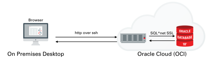
This workbook is divided into two sections the first is a quick guide to setting up Jupyter Lab (Python Notebooks) such that it can connect to a database running inside of OCI, in this case an ATP instance. The second section uses the JSON python driver to connect to the database to run a few tests. This notebook is largely a reminder to myself on how to set this up but hopefully it will be useful to others.
Setting up Python 3.6 and Jupyter Lab on our compute instance
I won't go into much detail on setting up ATP or ADW or creating a IaaS server. I covered that process in quite a lot of detail here. We'll be setting up something similar to the following
Once you've created the server You'll need to logon to the server with the details found on the compute instances home screen. You just need to grab it's IP address to enable you to logon over ssh.
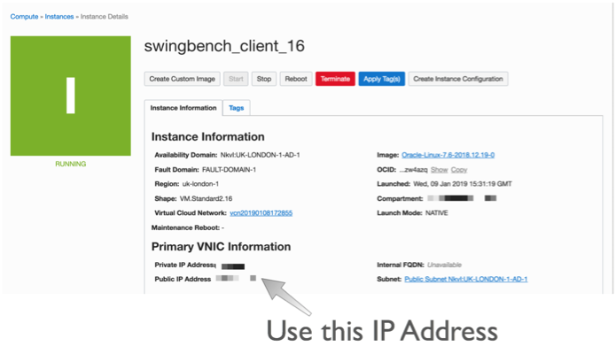
The next step is to connect over ssh to with a command similar to
ssh opc@132.146.27.111
Enter passphrase for key '/Users/dgiles/.ssh/id_rsa':
Last login: Wed Jan  9 20:48:46 2019 from host10.10.10.1
In the following steps we'll be using python so we need to set up python on the server and configure the needed modules. Our first step is to use yum to install python 3.6 (This is personal preference and you could stick with python 2.7). To do this we first need to enable yum and then install the environment. Run the following commands
sudo yum -y install yum-utils
sudo yum-config-manager --enable ol7_developer_epel
sudo yum install -y python36
python3.6 -m venv myvirtualenv
source myvirtualenv/bin/activate
This will install python and enable a virtual environment for use (our own Python sand pit). You can make sure that python is installed by simply typing python3.6 ie.
$> python3.6
Python 3.6.3 (default, Feb  1 2018, 22:26:31)
[GCC 4.8.5 20150623 (Red Hat 4.8.5-16)] on linux
Type "help", "copyright", "credits" or "license" for more information.
>>> quit()
Make sure you type quit() to leave the REPL environment.
We now need to install the needed modules. You can do this one by one or simply use the following file requirements.txt and run the following command
pip -p requirements.txt
This will install all of the need python modules for the next step which is to start up Jupyter Lab.
Jupyter Lab is an interactive web based application that enables you do interactively run code and document the process at the same time. This blog is written in it and the code below can be run once your environment is set up. Vists the website to see more details.
To start jupyer lab we run the following command.
nohup jupyter-lab --ip=127.0.0.1 &Be aware that this will only work if you have activated you virtual environment. In out instance we did this with with the command source myvirtualenv/bin/activate. At this point the jupyter-lab is running in the background and and is listening (by default) on port 8888. You could start a desktop up and use VNC to view the output. However I prefer to redirect the output to my own desktop over ssh. To do this you'll need to run the following ssh command from your desktop
ssh -N -f -L 5555:localhost:8888 opc@132.146.27.111
Replacing the IP address above with the one for your compute instance
This will redirect the output of 8888 to port 5555 on your destop. You can then connect to it by simply going to the following url http://localhost:5555. After doing this you should see a screen asking you input a token (you'll only need to do this once). You can find this token inside of the nohup.out file running on the compute instance. It should be near the top of the file and should look something like
[I 20:49:12.237 LabApp] http://127.0.0.1:8888/?token=216272ef06c7b7cb3fa8da4e2d7c727dab77c0942fac29c8
Just copy the text after "token=" and paste it in to the dialogue box. After completing that step you should see something like this
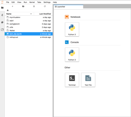
You can now start creating your own notebooks or load this one found here. I'd visit the website to familiarise yourself on how the notebooks work.
Using Python and the JSON SODA API
This section will walk through using The SODA API with Python from within the Jupyter-lab envionment we set up in the previous section. The SODA API is a simple object API that enables developers persist and retrieve JSON documents held inside of the Oracle Database. SODA drivers are available for Java, C, REST, Node and Python.
You can find the documentation for this API here
To get started we'll need to import the need the following python modules
import cx_Oracle
import keyring
import os
import pandas as pd
We now need to set the location of the directory containing the wallet to enable us to connect to the ATP instance. Once we've done that we can connect to the Oracle ATP instance and get a SODA object to enable us to work with JSON documents. NOTE : I'm using the module keyring to hide the password for my database. You should replace this call with the password for your user.
os.environ['TNS_ADMIN'] = '/home/opc/Wallet'
connection = cx_Oracle.connect('json', keyring.get_password('ATPLondon','json'), 'sbatp_tpurgent')
soda = connection.getSodaDatabase()
We now need to create JSON collection and if needed add any additional indexes which might accelerate data access.
try:
    collection = soda.createCollection("customers_json_soda")
    collection.createIndex({ "name"   : "customer_index",
                          "fields" : [ { "path"     : "name_last",
                          "datatype" : "string"}]})
except cx_Oracle.DatabaseError as ex:
    print("It looks like the index already exists : {}".format(ex))
We can now add data to the collection. Here I'm inserting the document into the database and retrieving it's key. You can find find some examples/test cases on how to use collections here
customer_doc = {"id"          : 1,
       "name_last"    : "Giles",
       "name_first"   : "Dom",
       "description"  : "Gold customer, since 1990",
       "account info" : None,
       "dataplan"     : True,
       "phones"       : [{"type" : "mobile", "number" : 9999965499},
                         {"type" : "home",   "number" : 3248723987}]}
doc = collection.insertOneAndGet(customer_doc)
connection.commit()
To fetch documents we could use SQL or Query By Example (QBE) as shown below. You can find further details on QBE here. In this example there should just be a single document. NOTE: I'm simply using pandas DataFrame to render the retrieved data but it does highlight how simple it is to use the framework for additional analysis at a later stage.
documents = collection.find().filter({'name_first': {'$eq': 'Dom'}}).getDocuments()
results = [document.getContent() for document in documents]
pd.DataFrame(results)
To update records we can use the replaceOne method.
document = collection.find().filter({'name_first': {'$eq': 'Dom'}}).getOne()
updated = collection.find().key(doc.key).replaceOne({"id"          : 1,
       "name_last"    : "Giles",
       "name_first"   : "Dominic",
       "description"  : "Gold customer, since 1990",
       "account info" : None,
       "dataplan"     : True,
       "phones"       : [{"type" : "mobile", "number" : 9999965499},
                         {"type" : "home",   "number" : 3248723987}]},)
connection.commit()
And just to make sure the change happened
data = collection.find().key(document.key).getOne().getContent()
pd.DataFrame([data])
And finally we can drop the collection.
try:
    collection.drop()
except cx_Oracle.DatabaseError as ex:
    print("We're were unable to drop the collection")
connection.close()
Python, Oracle_cx, Altair and Jupyter Notebooks
Simple Oracle/Jupyter/Keyring/Altair Example
In this trivial example we'll be using Jupyter Lab to create this small notebook of Python code. We will see how easy it is to run SQL and analyze those results. The point of the exercise here isn't really the SQL we use but rather how simple it is for developers or analysts who prefer working with code rather than a full blown UI to retrieve and visualise data.
For reference I'm using Python 3.6 and Oracle Database 12c Release 2. You can find the source here
First we'll need to import the required libraries. It's likely that you won't have them installed on your server/workstation. To do that use the following pip command "pip install cx_Oracle keyring pandas altair jupyter jupyter-sql". You should have pip installed and probably be using virtualenv but if you don't I'm afraid that's beyond the scope of this example. Note whilst I'm not importing jupyter and jupyter-sql in this example they are implicitly used.
import cx_Oracle
import keyring
import pandas as pd
import altair as alt
We will be using the magic-sql functionality inside of jupyter-lab. This means we can trivially embed SQL rather than coding the cusrsors and fetches we would typically have to do if we were using straight forward cx_Oracle. This uses the "magic function" syntax" which start with "%" or "%%". First we need to load the support for SQL
%load_ext sql
Next we can connect to the local docker Oracle Database. However one thing we don't want to do with notebooks when working with server application is to disclose our passwords. I use the python module "keyring" which enables you to store the password once in a platform appropriate fashion and then recall it in code. Outside of this notebook I used the keyring command line utility and ran "keyring set local_docker system". It then prompted me for a password which I'm using here. Please be careful with passwords and code notebooks. It's possible to mistakenly serialise a password and then potentially expose it when sharing notebooks with colleagues.
password = keyring.get_password('local_docker','system')
We can then connect to the Oracle Database. In this instance I'm using the cx_Oracle Diriver and telling it to connect to a local docker database running Oracle Database 12c (12.2.0.1). Because I'm using a service I need to specify that in the connect string. I also substitute the password I fetched earlier.
%sql oracle+cx_oracle://system:$password@localhost/?service_name=soe
I'm now connected to the Oracle database as the system user. I'm simply using this user as it has access to a few more tables than a typical user would. Next I can issue a simple select statement to fetch some table metadata. the %%sql result << command retrieves the result set into the variable called result
%%sql result <<
select table_name, tablespace_name, num_rows, blocks, avg_row_len, trunc(last_analyzed)
from all_tables
where num_rows  > 0
and tablespace_name is not null
In Python a lot of tabular manipulation of data is performed using the module Pandas. It's an amazing piece of code enabling you to analyze, group, filter, join, pivot columnar data with ease. If you've not used it before I strongly reccomend you take a look. With that in mind we need to take the resultset we retrieved and convert it into a DataFrame (the base Pandas tabular structure)
result_df = result.DataFrame()
We can see a sample of that result set the the Panada's head function
result_df.head()
All very useful but what if wanted to chart how many tables were owned by each user. To do that we could of course use the charting functionlty of Pandas (and Matplotlib) but I've recently started experimenting with Altair and found it to make much more sense when define what and how to plot data. So lets just plot the count of tables on the X axis and the tablespace name on the Y axis.
alt.Chart(result_df).mark_bar().encode(
    x='count()',
    y='tablespace_name',
)

Altair makes much more sense to me as a SQL user than some of the cryptic functionality of Matplotlib. But the chart looks really dull. We can trvially tidy it up a few additonal commands
alt.Chart(result_df).mark_bar().encode(
    x=alt.Y('count()', title='Number of tables in Tablespace'),
    y=alt.Y('tablespace_name', title='Tablespace Name'),
    color='tablespace_name'
).properties(width=600, height= 150, title='Tables Overview')

Much better but Altair can do significantly more sophisticated charts than a simple bar chart. Next lets take a look at the relationship between the number of rows in a table and the blocks required to store them. It's worth noting that this won't, or at least shouldn't, produce any startling results but it's a useful plot on a near empty database that will give use something to look at. Using another simple scatter chart we get the following
alt.Chart(result_df).mark_point().encode(
    y = 'num_rows',
    x = 'blocks',
).properties(width=600)

Again it's a near empty database and so there's not much going on or at least we have a lot of very small tables and a few big ones. Lets use a logarithmic scale to spread things out a little better and take the oppertunity to brighten it up
alt.Chart(result_df).mark_point().encode(
    y = alt.Y('num_rows',scale=alt.Scale(type='log')),
    x = alt.X('blocks', scale=alt.Scale(type='log')),
    color = 'tablespace_name',
    tooltip=['table_name']
).properties(width=600)

Much better... But Altair and the libraries it uses has a another fantastic trick up its sleeve. It can make the charts interactive (zoom and pan) but also enable you to select data in one chart and have it reflected in another. To do that we use a "Selection" object and use this to filter the data in a second chart. Lets do this for the two charts we created. Note you'll need to have run this notebook "live" to see the interactive selection.
interval = alt.selection_interval()

chart1 = alt.Chart(result_df).mark_point().encode(
    y = alt.Y('num_rows',scale=alt.Scale(type='log')),
    x = alt.X('blocks', scale=alt.Scale(type='log')),
    color = 'tablespace_name',
    tooltip=['table_name']
).properties(width=600, selection=interval)

chart2 = alt.Chart(result_df).mark_bar().encode(
    x='count()',
    y='tablespace_name',
    color = 'tablespace_name'
).properties(width=600, height= 150).transform_filter(
    interval
)

chart1 & chart2

And thats it. I'll be using this framework to create a few additional examples in the coming weeks.
The following shows what you would have seen if you had been running the notebook code inside of a browser
Making the alert log just a little more readable
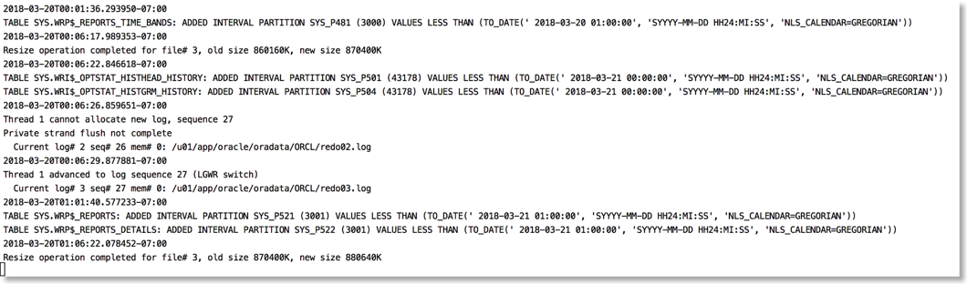
But what if you are only looking after one or two or just testing something out? Well the most common solution is to simply tail the alert log file.
The only issue is that it's not the most exciting thing to view, this of course could be said for any terminal based text file. But there are things you can do to make it easier to parse visually and improve your chances of catching an unexpected issue.
The approach I take is to push the alert log file through python and use the various libraries to brighten it up. It's very easy to go from this (tail -f)
To this
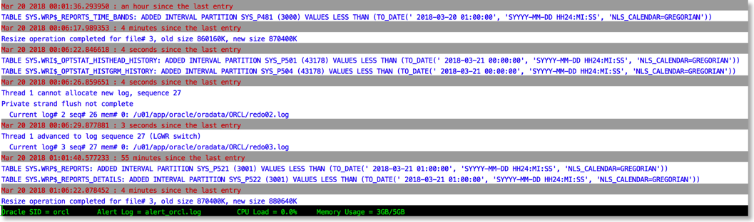
The reason this works is that python provides a rich set of libraries which can add a little bit of colour and formatting to the alert file.
You can find the code to achieve this in the gist below
Just a quick note on installing this. You'll need either python 2.7 or 3 available on your server.
I'd also recommend installing pip and then the following libraries
pip install humanize psutil colorama python-dateutil
After you've done that it's just a case of running the script. If you have $ORACLE_BASE and $ORACLE_SID set the library will try and make a guess at the location of the alert file. i.e
python alertlogparser.py
But if that doesn't work or you get an error you can also explicitly specify the location of the alert log with something like
python alertlogparser.py -a $ORACLE_BASE/diag/rdbms/orcl/orcl/trace/alert_orcl.log
This script isn't supposed to be an end product just a simple example of what can be achieved to make things a little easier. And whilst I print information like CPU load and Memory there's nothing to stop you from modifying the script to display the number of warnings or errors found in the alert log and update it things change. Or if you really want to go wild implement something similar but a lot more sophisticated using python and curses
The age of "Terminal" is far from over….
Installing Python 2.7 in local directory on Oracle Bare Metal Cloud
#make localdirectory to install python i.e.
mkdir python

#make sure latest libs needs for python are installed
sudo yum install openssl openssl-devel
sudo yum install zlib-devel

#Download latest source i.e. Python-2.7.13.tgz and uncompress
tar xvfz Python-2.7.13.tgz

cd Python-2.7.13
#configure python for local install
config --enable-shared --prefix=/home/opc/python --with-libs=/usr/local/lib
make; make install

#python 2.7.13 is now installed but isn't currently being used (2.6 is still the default)

#get pip
curl https://bootstrap.pypa.io/get-pip.py -o get-pip.py
#install pip (this will still be installed with 2.6)
sudo python get-pip.py
#install virtualenv
sudo pip install virtualenv
#create a virtualenv using the newly installed python
virtualenv -p /home/opc/python/bin/python myvirtualenv
#activate it
source myvirtualenv/bin/activate
#install packages…
pip install cx_Oracle
Changing the size of redo logs in python
The following code works it's way through the redo log files drops one thats inactive and then simply recreates it. It finished when it's set all of the redo to the right size.
Running the script is simply a case of running it with the parameters shown below
python ChangeRedoSize -u sys -p welcome1 -cs myserver/orclcdb --size 300
Note : the user is the sysdba of the container database if you are using the multitenant arhcitecture and the size is in Mega Bytes.
You should then see something similar to the following
Current Redo Log configuration
+-----------+------------+--------------+-----------+---------------+----------+
| Group No. | Thread No. | Sequence No. | Size (MB) | No of Members |  Status  |
+-----------+------------+--------------+-----------+---------------+----------+
|     1     |     1      |     446      | 524288000 |       1       | INACTIVE |
|     2     |     1      |     448      | 524288000 |       1       | CURRENT  |
|     3     |     1      |     447      | 524288000 |       1       |  ACTIVE  |
+-----------+------------+--------------+-----------+---------------+----------+
alter system switch logfile
alter system switch logfile
alter database drop logfile group 2
alter database add logfile group 2 size 314572800
alter system switch logfile
alter database drop logfile group 1
alter database add logfile group 1 size 314572800
alter system switch logfile
alter system switch logfile
alter system switch logfile
alter system switch logfile
alter database drop logfile group 3
alter database add logfile group 3 size 314572800
alter system switch logfile
All logs correctly sized. Finishing...
New Redo Log configuration
+-----------+------------+--------------+-----------+---------------+----------+
| Group No. | Thread No. | Sequence No. | Size (MB) | No of Members |  Status  |
+-----------+------------+--------------+-----------+---------------+----------+
|     1     |     1      |     455      | 314572800 |       1       |  ACTIVE  |
|     2     |     1      |     454      | 314572800 |       1       | INACTIVE |
|     3     |     1      |     456      | 314572800 |       1       | CURRENT  |
+-----------+------------+--------------+-----------+---------------+----------+
Interpolating data with Python
So as usual for this time of year I find myself on vacation with very little to do. So I try and find personal projects that interest me. This is usually a mixture of electronics and mucking around with software in a way that I don't usally find the time for normally. One of projects is my sensor network.
I have a number of Raspberry Pi's around my house and garden that take measurements of temperature, humidity, pressure and light. They hold the data locally and then periodically upload them to a central server (another Raspberry Pi) where they are aggregated. However for any number of reasons (usally a power failure) the raspberrypi's occasionally restart and are unable to join the network. This means that some of their data is lost. I've improved their resiliance to failure and so it's a less common occurance but it's still possible for it to happen. When this means I'm left with some ugly gaps in an otherwise perfect data set. It's not a big deal but it's pretty easy to fix. Before I begin, I acknolwedge that I'm effectively "making up" data to make graphs "prettier".
In the following code notebook I'll be using Python and Pandas to tidy up the gaps.
To start with I need to load the libraries to process the data. The important ones are included at the start of the imports. The rest from "SensorDatabaseUtilities" aren't really relevant since they are just helper classes to get data from my repository
import matplotlib.pyplot as plt
from matplotlib import style
import pandas as pd
import matplotlib
import json
from pandas.io.json import json_normalize
# The following imports are from my own Sensor Library modules and aren't really relevant
from SensorDatabaseUtilities import AggregateItem
from SensorDatabaseUtilities import SensorDatabaseUtilities
# Make sure the charts appear in this notebook and are readable
%matplotlib inline
matplotlib.rcParams['figure.figsize'] = (20.0, 10.0)
The following function is used to convert a list of JSON documents (sensor readings) into a Pandas DataFrame. It then finds the minimum and maximum dates and creates a range for that period. It uses this period to find any missing dates. The heavy lifting of the function uses the reindex() function to insert new entries whilst at the same time interpolating any missing values in the dataframe. It then returns just the newly generated rows
def fillin_missing_data(sensor_name, results_list, algorithm='linear', order=2):
    # Turn list of json documents into a json document
    results = {"results": results_list}
    # Convert JSON into Panda Dataframe/Table
    df = json_normalize(results['results'])
    # Convert Date String to actual DateTime object
    df['Date'] = pd.to_datetime(df['Date'])
    # Find the max and min of the Data Range and generate a complete range of Dates
    full_range = pd.date_range(df['Date'].min(), df['Date'].max())
    # Find the dates that aren't in the complete range
    missing_dates = full_range[~full_range.isin(df['Date'])]
    # Set the Date to be the index
    df.set_index(['Date'], inplace=True)
    # Reindex the data filling in the missing date and interpolating missing values
    if algorithm in ['spline', 'polynomial'] :
        df = df.sort_index().reindex(full_range).interpolate(method=algorithm, order=order)
    elif algorithm in ['ffill', 'bfill']:
        df = df.sort_index().reindex(full_range, method=algorithm)
    else:
        df = df.sort_index().reindex(full_range).interpolate(method=algorithm)
    # Find the dates in original data set that have been added
    new_dates = df[df.index.isin(missing_dates)]
    # Create new aggregate records and insert them into the database
    # new_dates.apply(gen_json,axis=1, args=[sensor_name])
    return new_dates
This function simply takes an array of JSON documents and converts them into a DataFrame using the Pandas json_normalize function. It provides us with the dataset that contains missing data i.e. an incomplete data set.
def json_to_dataframe(results_list):
    # Turn list of json documents into a json dodument
    results = {"results": results_list}
    # Convert JSON into Panda Dataframe/Table
    df = json_normalize(results['results'])
    return df
The first step is to pull the data from the database. I'm using some helper functions to do this for me. I've also selected a date range where I know I have a problem.
utils = SensorDatabaseUtilities('raspberrypi', 'localhost')
data = utils.getRangeData('20-jan-2015', '10-feb-2015')
# The following isn't need in the code but is included just to show the structure of the JSON Record
json.dumps(data[0])
Next simply convert the list of JSON records into a Pandas DataFrame and set it's index to the "Date" Column. NOTE : Only the first 5 records are shown
incomplete_data = json_to_dataframe(data)
# Find the range of the data and build a series with all dates for that range
full_range = pd.date_range(incomplete_data['Date'].min(), incomplete_data['Date'].max())
incomplete_data['Date'] = pd.to_datetime(incomplete_data['Date'])
incomplete_data.set_index(['Date'], inplace=True)
# Show the structure of the data set when converted into a DataFrame
incomplete_data.head()
The following step isn't needed but simply shows the problem we have. In this instance we are missing the days for Janurary 26th 2015 to Janurary 30th 2015
#incomplete_data.set_index(['Date'], inplace=True)
problem_data = incomplete_data.sort_index().reindex(full_range)
axis = problem_data['AverageTemperature'].plot(kind='bar')
axis.set_ylim(18,22)
plt.show()

Pandas offers you a number of approaches for interpolating the missing data in a series. They range from the simple method of backfilling or forward filling values to the more powerful approaches of methods such as "linear", "quadratic" and "cubic" all the way through to the more sophisticated approaches of "pchip", "spline" and "polynomial". Each approach has its benefits and disadvantages. Rather than talk through each it's much simpler to show you the effect of each interpolation on the data. I've used a line graph rather than a bar graph to allow me to show all of the approaches on a single graph.
interpolation_algorithms = ['linear', 'quadratic', 'cubic', 'spline', 'polynomial', 'pchip', 'ffill', 'bfill']

fig, ax = plt.subplots()
for ia in interpolation_algorithms:
    new_df = pd.concat([incomplete_data, fillin_missing_data('raspberrypi', data, ia)])
    ax = new_df['AverageTemperature'].plot()

handles, not_needed = ax.get_legend_handles_labels()
ax.legend(handles, interpolation_algorithms, loc='best')

plt.show()

Looking at the graph it appears that either pchip (Piecewise Cubic Hermite Interpolating Polynomial) or Cubic interpolation is going to provide the best approximation for the missing values in my data set. This is largely subjective because these are "made up values" but I believe either of these approaches provide values that are closest to what the data could have been.
The next step is to apply one to the incomplete data set and store it back in the database
complete_data = pd.concat([incomplete_data, fillin_missing_data('raspberrypi', data, 'pchip')])

axis = complete_data.sort_index()['AverageTemperature'].plot(kind='bar')
axis.set_ylim(18,22)
plt.show()

And thats it. I've made the code much more verbose that it needed to be purely to demonstrate the point. Pandas makes it very simple to patch up a data set.
Java Version Performance
Now before we go any further it’s worth pointing out this was a trivial test and my results might not be representative of what you or anyone else might find.
My environment was
iMac (Retina 5K, 27-inch, Late 2014), 4 GHz Intel Core i7, 32 GB 1600 MHz DDR3 with a 500GB SSD
Oracle Database 12c (12.1.0.2) with the January Patch Bundle running in a VM with 8GB of memory.
The test is pretty simple but might have an impact on your choice of JVM when generating a lot of data (TB+) with swingbench. I simply created a 1GB SOE with the oewizard. This is a pretty CPU intensive operation for the entire stack : swingbench, the jdbc drivers and the database. The part of the operation that should be most effected by the performance of the JVM is the “Data Generation Step”.
So enough talk what impact did the JVM version have?

Now the numbers might not be earth shattering but it’s nice to know a simple upgrade of the JVM can result in nearly a 25% improvement in performance of a CPU/database intensive batch job. I expect these numbers to go up as I optimise some of the logic to take advantage of Java8 specific functionality.
PDF Generation of report files
All you need to do is to run swingbench and from the menu save the summary results.
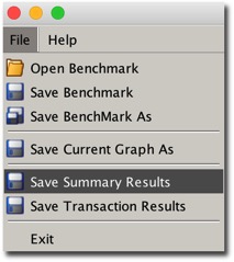
Minibench and charbench will automatically create a results config file in the local directory after a benchmark run. The file that’s created will typically start with “result” and it should look something like this.
[bin]$ ls ccwizard.xml coordinator oewizard shwizard.xmlbmcompare charbench data oewizard.xml swingbenchccconfig.xml clusteroverview debug.log results.xml swingconfig.xmlccwizard clusteroverview.xml minibench shwizardAll you need to do after this is to run the “results2pdf command
[bin]$ ./results2pdf -c results2pdf
There’s really only 2 command line options
[bin]$ ./results2pdf -husage: parameters: -c
The resultant file will contain tables and graphs. The type of data will depend heavily on the type of stats collected in the benchmark. For the richest collection you should enable
- Full stats collection
- Database statistics collection
- CPU collection
An example of the output can be found here.

I plan to try and have the resultant pdf generated and displayed at the end of every bench mark. I’ll include this functionality in a future build.