Oracle SODA Python Driver and Jupyter Lab
Oracle SODA Python Driver and Jupyter Lab
This workbook is divided into two sections the first is a quick guide to setting up Jupyter Lab (Python Notebooks) such that it can connect to a database running inside of OCI, in this case an ATP instance. The second section uses the JSON python driver to connect to the database to run a few tests. This notebook is largely a reminder to myself on how to set this up but hopefully it will be useful to others.
Setting up Python 3.6 and Jupyter Lab on our compute instance
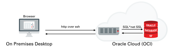
I won't go into much detail on setting up ATP or ADW or creating a IaaS server. I covered that process in quite a lot of detail here. We'll be setting up something similar to the following
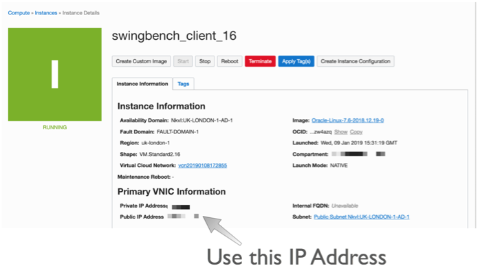
Once you've created the server You'll need to logon to the server with the details found on the compute instances home screen. You just need to grab it's IP address to enable you to logon over ssh.
The next step is to connect over ssh to with a command similar to
ssh opc@132.146.27.111
Enter passphrase for key '/Users/dgiles/.ssh/id_rsa':
Last login: Wed Jan  9 20:48:46 2019 from host10.10.10.1
In the following steps we'll be using python so we need to set up python on the server and configure the needed modules. Our first step is to use yum to install python 3.6 (This is personal preference and you could stick with python 2.7). To do this we first need to enable yum and then install the environment. Run the following commands
sudo yum -y install yum-utils
sudo yum-config-manager --enable ol7_developer_epel
sudo yum install -y python36
python3.6 -m venv myvirtualenv
source myvirtualenv/bin/activate
This will install python and enable a virtual environment for use (our own Python sand pit). You can make sure that python is installed by simply typing python3.6 ie.
$> python3.6
Python 3.6.3 (default, Feb  1 2018, 22:26:31)
[GCC 4.8.5 20150623 (Red Hat 4.8.5-16)] on linux
Type "help", "copyright", "credits" or "license" for more information.
>>> quit()
Make sure you type quit() to leave the REPL environment.
We now need to install the needed modules. You can do this one by one or simply use the following file requirements.txt and run the following command
pip -p requirements.txt
This will install all of the need python modules for the next step which is to start up Jupyter Lab.
Jupyter Lab is an interactive web based application that enables you do interactively run code and document the process at the same time. This blog is written in it and the code below can be run once your environment is set up. Vists the website to see more details.
To start jupyer lab we run the following command.
nohup jupyter-lab --ip=127.0.0.1 &Be aware that this will only work if you have activated you virtual environment. In out instance we did this with with the command source myvirtualenv/bin/activate. At this point the jupyter-lab is running in the background and and is listening (by default) on port 8888. You could start a desktop up and use VNC to view the output. However I prefer to redirect the output to my own desktop over ssh. To do this you'll need to run the following ssh command from your desktop
ssh -N -f -L 5555:localhost:8888 opc@132.146.27.111
Replacing the IP address above with the one for your compute instance
This will redirect the output of 8888 to port 5555 on your destop. You can then connect to it by simply going to the following url http://localhost:5555. After doing this you should see a screen asking you input a token (you'll only need to do this once). You can find this token inside of the nohup.out file running on the compute instance. It should be near the top of the file and should look something like
[I 20:49:12.237 LabApp] http://127.0.0.1:8888/?token=216272ef06c7b7cb3fa8da4e2d7c727dab77c0942fac29c8
Just copy the text after "token=" and paste it in to the dialogue box. After completing that step you should see something like this
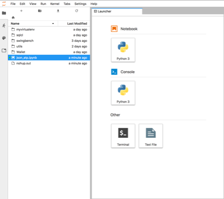
You can now start creating your own notebooks or load this one found here. I'd visit the website to familiarise yourself on how the notebooks work.
Using Python and the JSON SODA API
This section will walk through using The SODA API with Python from within the Jupyter-lab envionment we set up in the previous section. The SODA API is a simple object API that enables developers persist and retrieve JSON documents held inside of the Oracle Database. SODA drivers are available for Java, C, REST, Node and Python.
You can find the documentation for this API here
To get started we'll need to import the need the following python modules
import cx_Oracle
import keyring
import os
import pandas as pd
We now need to set the location of the directory containing the wallet to enable us to connect to the ATP instance. Once we've done that we can connect to the Oracle ATP instance and get a SODA object to enable us to work with JSON documents. NOTE : I'm using the module keyring to hide the password for my database. You should replace this call with the password for your user.
os.environ['TNS_ADMIN'] = '/home/opc/Wallet'
connection = cx_Oracle.connect('json', keyring.get_password('ATPLondon','json'), 'sbatp_tpurgent')
soda = connection.getSodaDatabase()
We now need to create JSON collection and if needed add any additional indexes which might accelerate data access.
try:
    collection = soda.createCollection("customers_json_soda")
    collection.createIndex({ "name"   : "customer_index",
                          "fields" : [ { "path"     : "name_last",
                          "datatype" : "string"}]})
except cx_Oracle.DatabaseError as ex:
    print("It looks like the index already exists : {}".format(ex))
We can now add data to the collection. Here I'm inserting the document into the database and retrieving it's key. You can find find some examples/test cases on how to use collections here
customer_doc = {"id"          : 1,
       "name_last"    : "Giles",
       "name_first"   : "Dom",
       "description"  : "Gold customer, since 1990",
       "account info" : None,
       "dataplan"     : True,
       "phones"       : [{"type" : "mobile", "number" : 9999965499},
                         {"type" : "home",   "number" : 3248723987}]}
doc = collection.insertOneAndGet(customer_doc)
connection.commit()
To fetch documents we could use SQL or Query By Example (QBE) as shown below. You can find further details on QBE here. In this example there should just be a single document. NOTE: I'm simply using pandas DataFrame to render the retrieved data but it does highlight how simple it is to use the framework for additional analysis at a later stage.
documents = collection.find().filter({'name_first': {'$eq': 'Dom'}}).getDocuments()
results = [document.getContent() for document in documents]
pd.DataFrame(results)
To update records we can use the replaceOne method.
document = collection.find().filter({'name_first': {'$eq': 'Dom'}}).getOne()
updated = collection.find().key(doc.key).replaceOne({"id"          : 1,
       "name_last"    : "Giles",
       "name_first"   : "Dominic",
       "description"  : "Gold customer, since 1990",
       "account info" : None,
       "dataplan"     : True,
       "phones"       : [{"type" : "mobile", "number" : 9999965499},
                         {"type" : "home",   "number" : 3248723987}]},)
connection.commit()
And just to make sure the change happened
data = collection.find().key(document.key).getOne().getContent()
pd.DataFrame([data])
And finally we can drop the collection.
try:
    collection.drop()
except cx_Oracle.DatabaseError as ex:
    print("We're were unable to drop the collection")
connection.close()